We observe an unknown function \(T\) through a set of \(n\) observation functionals \(\{\mathrm{L}_i\}_{i=1}^n\), where each \(\mathrm{L}_i\) maps \(T\) to its integral on \([a,b]\), weighted by some observation function \(g_i\). For each \(i\in\{1,\ldots, n\}\) the \(i\)th functional \(\mathrm{L}_i\), when applied to \(T\), produces the observation \(\nu_i\) as follows:
With nondegenerate \(g_i\), these \(\mathrm{L}_i\) are bounded, linear observation functionals. We could therefore define a wiggliness penalty on a Sobolev space associated with this index set \(\mathcal{X}=[a,b]\), defined so as to be sufficiently expressive to house the observation functionals' Riesz representers, and use the representer theorem of Grace Wahba and George Kimeldorf to write the reconstructed estimate of \(T\) as a linear combination of these Riesz representers. By a simple orthogonality argument, this reconstructed estimate of \(T\) will either be the function in the infinite-dimensional Sobolev space that, among those that produce the same set of observations, has minimal wiggliness penalty (exact interpolation) or the function in that space that minimizes a weighted sum of its disagreement with the observations and the wiggliness functional (smoothing). Unfortunately, this is difficult to implement on a computer for many applications.
We instead approximate this infinite-dimensional Sobolev space as the span of a finite set of \(L\) spline basis functions. (It can, after all, be seen as the closure of the span of such functions—the representers of evaluation at each point over the continuum of the index set \([a,b]\).) Here we use the B-spline basis functions.
Accordingly, we approximate our unknown function \(T\) as a weighted sum of \(L\) B-spline basis functions \(\{\phi_i\}_{j=1}^L\):
\[T(x) = \sum_{j=1}^L \alpha_j \phi_j(x).\]
⚠ Note
Here we are effectively assuming that \(T\) is a spline, or can profitably be modeled as such. Fitting this expansion from discrete samples is quite unlike the Shannon-Whittaker cardinal sinc expansion (see, e.g., [1], eq. (5)), which recovers exactly the discrete data, as the sinc pulses are 1 at one sample point and 0 at all the others. The spline model, sampled at these discrete locations, smooths the original discrete data—even if there are basis functions centered at each discrete sample point.
There are many ways to fit a spline model to data. The most common approach is to choose spline weights \(\{\alpha_j\}_{j=1}^L\) so that the spline model (2) minimizes the squared error at the discrete samples. This is not always the best approach for ensuring the accuracy of our integral.
When comparing the continuous model (2) to a data source, often discrete, there are therefore two sources of error: the smoothing of the samples, and incorrect interpolation (aliasing). By contrast, the Shannon-Whittaker interpolation formula suffers only from the second defect. If the underlying continuous function sampled resides in an appropriate Paley-Wiener RKHS of bandlimited signals and is sampled at the Nyquist rate, the infinite Shannon-Whittaker expansion recovers the correct underlying continuous function. If the samples are inadequately spaced, the continuous function will still correctly reproduce these samples but will interpolate incorrectly: it will exhibit aliasing.
Thus, the spline model (2) is an approximation.
Then for each \(i\in\{1,\ldots,n\}\), the \(i\)th observation functional, applied to (our spline-reconstructed signal) \(T\), yields the observation
The value \(\nu_i\) assumed by the functional \(\mathrm{L}_i\), when applied to \(T\), is a weighted sum of the values that very functional assumes when applied to the \(L\) basis functions \(\{\phi_i\}_{i=1}^L\).
At first glance, this seems silly. We've turned one integral, of the product \(T \cdot g_i\), into \(L\) integrals, of \(\phi_j\cdot g_i\) for each \(j=1,\ldots, L\). If \(T\) can be well-approximated as a weighted sum of these \(L\) basis functions, it must be well-behaved. Why not simply compute integral (1) directly?
Well, we are not actually working directly. We are solving an inverse problem, to reconstruct \(T\) from a set of observations. It can be easier in many cases to recover the weights \(\{\alpha_i\}_{i=1}^L\) on the decomposition (2) than it is to reconstruct \(T\) through other means of discretizing the integral (1)—for instance, as a Riemann sum rather than our weighted sum of observation functionals applied to spline basis functions.
To compute the \(\mathrm{L}_i(\phi_j)\), we use a Monte Carlo method.
where the scaling factor \(\mu_j = \int_{-\infty}^\infty \phi_j(u) \mathop{}\!\mathrm{d}u\) turns our basis function \(\phi_j\) into a probability density function. To compute this expectation, we need to draw samples from the basis function \(\phi_j\), normalized as a probability distribution \(p_j\).
B-splines were introduced, or, rather, first seen as important enough to merit their being named, by Isaac Jacob Schoenberg in 1946 [1]. He used them to form interpolants of equidistant data; this was generalized almost immediately to nonuniform knots or data points by Haskell Curry. Curry's name is not often associated with splines, in part because the paper containing his insight took 20 years to get published [2]; this may be surprising, but the contribution fits in with his body of work. Schoenberg remarks that the B-spline basis functions—expressed as divided differences of the ramp function (or reLu, as fashion dictates)—were "essentially" a result of Laplace's work, because the \(k\)th B-spline basis function \(M_k\) is the distribution of error in the sum \(Y\) of \(k\) random variables \(Y = X_1+\ldots + X_k\) if we replace each random variable \(X_i\) by its value rounded to the nearest integer (see [1], section 3.17). They had also arisen in the interpolation context (where probabilistic arguments are quite common: e.g., the proof that the Bernstein polynomial interpolant of some continuous function \(f\) on \([0,1]\), \(M_n(x) = \sum_{\nu=0}^n f\left(\frac{\nu}{n}\right)\binom{n}{\nu}x^\nu(1-x)^{n-\nu}\), converges uniformly toward \(f\) on \([0,1]\) as \(n\to \infty\) follows by considering a game where the reward for winning \(\nu\) trials out of \(n\) is \(f\left(\frac{\nu}{n}\right)\), along with the law of large numbers and continuity of \(f\)); Carl de Boor notes that Jean Favard had used B-splines in interpolation earlier [3]-[4].
Given knots \(\xi_1 \leq \ldots \leq \xi_n\) and order \(k\), the B-spline basis function \(N_{i,p}\) can be defined using the Cox-de Boor formula:
Thus, if we are rounding a uniform random variable to the nearest integer, \(I\) represents a uniform distribution over the quantization error.
We let \(M_1 = I\) and for any integer \(k\geq 2, M_k = I \ast M_{k-1}\), where \(\ast\) represents convolution: for any \(f, g\) in \(L^1(\mathbb{R})\), we can write
Since convolution in the time domain corresponds to the multiplication of spectra and since the Fourier transform (in the non-unitary, angular form with \(2\pi\) factor in the inverse transform) of \(I\) is given by
These are called cardinal B-spline basis functions, for they are defined by a knot vector with spacing 1. In other words, \(M_k(x) = N_{1,k}(x)\), where \(N_{1,k}\) is defined by the Cox-de Boor recursion (5) on the knots \(\xi_1=-\frac{k}{2}, \xi_2=-\frac{k}{2}+1, \ldots, \xi_{k} = \frac{k}{2}-1\).
The profile of the cardinal contains curves quite similar to the B-splines of several different orders. (Image source: Matt Bango, who released it into the public domain with a CC0 license.)
Anyone who has taken a signal processing course can immediately see that, as the convolution of a rectangular function with itself, \(M_2\) is a triangular function:
This function is symmetric and continuous, with a continuous derivative and second derivative, and a discontinuous but square-integrable third derivative. As with \(M_1\) through \(M_3\) (and beyond, since the convolution of two PDFs is a PDF), it integrates to 1 and is a valid PDF.
Note that some authors (e.g., [5]) define the cardinal B-splines so that \(\text{support}(M_k) = [0, k]\).
One way to draw samples from a random variable \(X\) with known CDF \(F_X\) is to use samples of a uniform random variable in [0,1], via the inverse-transform sampling trick. Since a CDF ranges between 0 and 1, if we can compute its (generalized) inverse (the PPF (probability point function, or quantile function) \(F^{-1}_X\) defined by \(F^{-1}_X(u) = \text{inf}\, \{ x\in\mathbb{R} \; | \; F_X(x) \geq u\}\)) we can implement the following procedure:
Obtain samples \(u_1, \ldots, u_n\) of independent, identically distributed random variables \(U_1,\ldots, U_n\), with each \(U_i \sim \text{Unif}(0,1)\) for \(i=1,\ldots, n\).
For each \(i=1,\ldots, n\), compute \(x_i = F_X^{-1}(u_i)\).
Return \(x_1,\ldots, x_n\).
The proof that this works is simple. It follows from the fact that CDFs are nondecreasing and càdlàg, so the following maneuver is permitted:
\[P(F_X^{-1}(u) \leq x) = P(u \leq F_X(x));\]
since \(\{u \; | \; F_X^{-1}(u)\leq x\} = \{u \;|\; u \leq F(x)\}\), and the samples \(u\) are distributed uniformly in [0,1], the probability that they are at most \(F_X(x)\) is exactly \(F_X(x)\).
The CDF of \(M_4\) is found by integrating (14), since the CDF \(F_X\) of a random variable \(X\) is related to its PDF \(f_X\) as follows: \(F_X(x) = \int_{-\infty}^x f_X(u)\mathop{}\!\mathrm{d}{u}.\) Suppose we have a random variable \(x\) such that \(f_X(x) = M_4(x)\). Then
\[F_X(x) = \int_{-\infty}^x M_4(u)\mathop{}\!\mathrm{d}{u} = \begin{cases} \frac{1}{24}\left(x+2\right)^4, & \text{ if } x\in[-2,-1);\\
\frac{1}{24}\left(-3x^4 -8x^3 + 16x +12\right), &\text{ if } x\in[-1,0);\\
\frac{1}{24}\left(3x^4-8x^3+16x+12\right), &\text{ if } x\in[0,1);\\
1-\frac{1}{24}\left(2-x\right)^4, &\text{ if } x\in[1,2);\\
0, &\text{ otherwise.}\end{cases}\]
Given a sample \(U=u\) of \(U\sim \text{Unif}(0,1)\), we can trivially solve \(u=F_X(x)\) when \(u\in\left[0,\frac{1}{24}\right)\) or \(u\in\left[\frac{23}{24},1\right]\), but if \(u\in\left[\frac{1}{24},\frac{1}{2}\right)\), we must solve a quartic equation with two complex roots for the smaller real root, which starts at -1 when \(u=\frac{1}{24}\) and slides over to \(0\) when \(u=\frac{1}{2}\). When \(u\in \left[\frac{1}{2}, \frac{23}{24}\right)\), we must find the larger of the two real roots, now sliding between 0 and 1. Thus,
\[F_X^{-1}(u) = \begin{cases}
-2+\sqrt[4]{24u}, &\text{ if } u \in \left[0,\frac{1}{24}\right);\\
\text{solve } -3x^4 -8x^3 +16x+(12-24u) \text{ for the root in $[-1,0)$}, &\text{ if } u\in\left[\frac{1}{24}, \frac{1}{2}\right);\\
\text{solve } 3x^4 -8x^3 +16x +(12-24u) \text{ for the root in $[0,1)$}, &\text{ if } u\in\left[\frac{1}{2}, \frac{23}{24}\right);\\
2-\sqrt[4]{24(1-u)}, &\text{ if } u \in \left[\frac{23}{24},1\right].
\end{cases}\]
The root can be found by typing the analytical solution to the quartic equation (not fun) or with any variant of Newton's method. The derivative of the quartic equation is extremely easy to evaluate and conditioning is not an issue: with a reasonable guess for the initial point, the derivative will not be near zero. In practice, other Monte Carlo methods would be much simpler and more efficient (rejection sampling works fine), but what the hey, it's quick enough to implement this. (Sorry Pythonistas, it's in julia, but it should be easy enough to follow.)
using MTH229, Plots, LaTeXStrings
## NEWTON'S METHOD FOR ROOT FINDING
"""vanilla newton's method"""
function newton(f, fp, x, tol=1e-14, niter=100)
xnew, xold = x, Inf
ynew, yold = f(xnew), Inf
i=0
while (i<100) && (abs(xnew-xold) > tol) && (abs(ynew-yold) > tol)
xold, yold = xnew, ynew
xnew = xold - yold/fp(xold)
ynew = f(xnew)
i += 1
end
if i>=100
error("Did not converge")
end
return xnew, ynew
end
## OUR FUNCTIONS AS INPUT TO NEWTON
"""for root-finding in equation (18), second case"""
function get_f1(u)
# CDF for u in [1/24, 1/2)
f1(x) = -3x^4 - 8x^3 + 16x + (12-24*u)
f1p(x) = -12x^3 - 24x^2 + 16
return f1, f1p
end
"""for root-finding in equation (18), third case"""
function get_f2(u)
# CDF for u in [1/2, 23/24)
f2(x) = 3x^4 - 8x^3 + 16x + (12-24*u)
f2p(x) = 12x^3 - 24x^2 + 16
return f2, f2p
end
## OUR INITIAL GUESSES FOR NEWTON
"""dumbest possible linear interpolation between roots, u in [1/24, 1/2)"""
function get_x1(u)
return -1+(u-1/24)/(0.5-1/24)
end
"""dumbest possible linear interpolation between roots, u in [1/2, 23/24)"""
function get_x2(u)
return (u-0.5)/(23/24-0.5)
end
## THE QUANTILE FUNCTION OF B4
"""equation (18)"""
function ppf_b4(u)
if 0 <= u < 1/24
return -2 + (24*u)^(1/4)
elseif 1/24 <= u < 1/2
x = get_x1(u)
f1, f1p = get_f1(u)
return newton(f1, f1p, x)[1]
elseif 1/2 <= u < 23/24
x = get_x2(u)
f2, f2p = get_f2(u)
return newton(f2, f2p, x)[1]
elseif 23/24 <= u <= 1
return 2 - (24*(1-u))^(1/4)
else
error("u must be in [0,1]")
end
end
## GENERATE 100,000 SAMPLES OF M_4
n=100000
us = rand(n)
samples = ppf_b4.(us)
## PLOT
default(fontfamily="Computer Modern", grid=false, dpi=600)
stephist(samples, label=L"M_4\; \mathrm{(histogram)}", normalize=:pdf, color=:dodgerblue1, lw=.8)
## COMPARE WITH THE ACTUAL CUBIC B-SPLINE, COMPUTED USING COX-DE BOOR
## Note: cardinal_bspline_theoretical is defined in the next code snippet
xs = -2:0.001:2
plot!(xs, cardinal_bspline_theoretical(xs,4,-2.0); label=L"M_4\; \mathrm{(pdf)}", color=:dodgerblue1, lw=.5, linestyle=:dash)
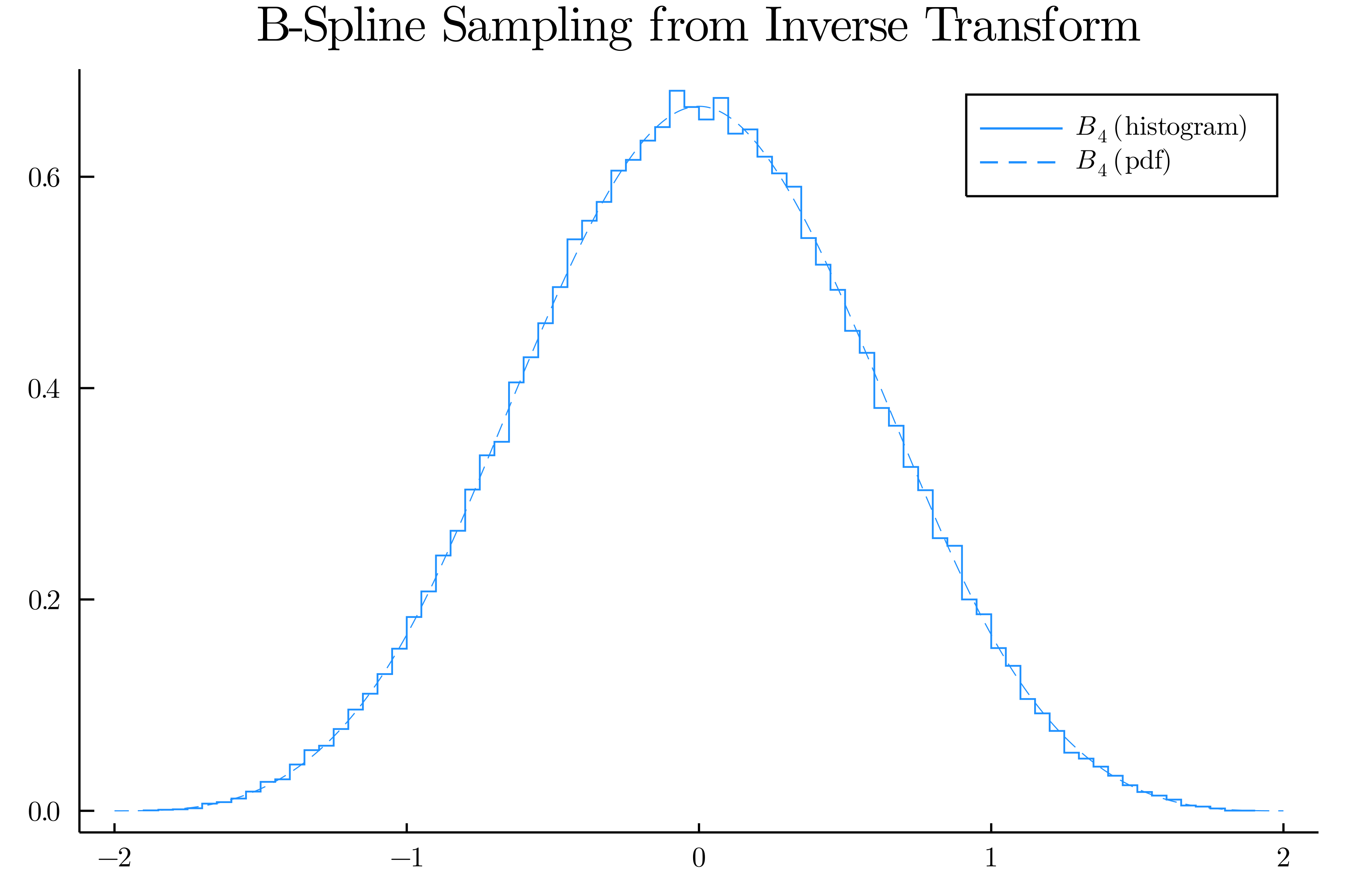
title!("B-Spline Sampling from Inverse Transform")
savefig("smirnov_sampler.png")
The figure produced by the code above, comparing the cardinal cubic B-spline function with inverse-transform sampling of the associated CDF.
This only works for cardinal B-splines, and not those with non-uniform knot spacing. If one were committed to using this sampling method, one could model a non-uniform spline basis function using a set of cardinal B-splines, I guess.
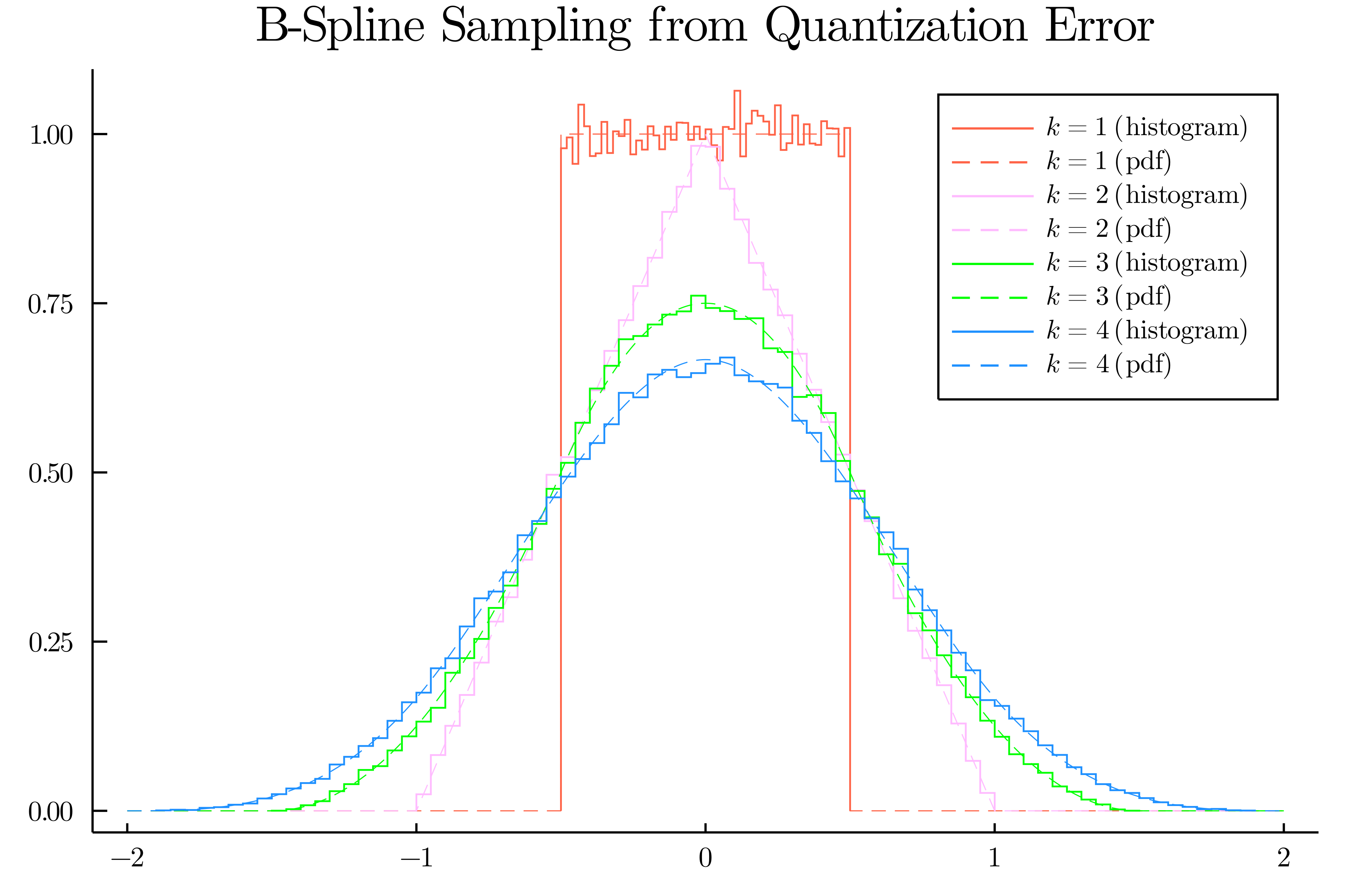
Since summing random variables convolves their PDFs, we can sample from \(M_2\)—or any cardinal B-spline—quite easily. The function cardinal_bspline_samples in the following code does just that. We compare the results with the PDF of the cardinal B-spline derived from the Cox-de Boor formula in cardinal_bspline_theoretical.
using Plots, LaTeXStrings

## Functions for generating samples of the density and evaluating the theoretical PDF

"""
	cardinal_bspline_samples(n,k)

	returns n samples from the cardinal (uniform knot spacing of 1) B-spline of order k (degree k-1),
	computed via the difference between the sum of k random variables and the sum of their rounded values

"""
function cardinal_bspline_samples(n::Integer, k::Integer)
    u = rand(Float64, (n,k)) # nxk array of samples of the uniform distribution, between 0 and 1
    r = round.(u) # elementwise rounding
    d = sum(r,dims=2)-sum(u,dims=2) # to get cardinal B-spline samples, compare the sum of the k random variables to their rounded values
    return d
end


"""
	cardinal_bspline_theoretical(x, k, l)

	evaluates the cardinal (uniform knot spacing of 1) B-spline of order k (degree k-1) at x, with left-most knot l;
	for a centered result, set the left-most knot l=-k/2
	note that this is implemented inefficiently: it's just the Cox-de Boor recursion

"""
function cardinal_bspline_theoretical(x, k::Integer, l::Float64)
    if k==1 # Cox-de Boor base case
        return ifelse.(l .<= x .< l+1, 1, 0)
    end
    return (x .- l)/abs(k-1).*cardinal_bspline_theoretical(x, k-1, l) + ((l+k) .- x)/abs(k-1).*cardinal_bspline_theoretical(x, k-1, l+1) # Cox-de Boor recursion
end

## Experiments and plotting

n = 100000 # number of samples to draw for each random variable in the sum associated with a given experiment
xs = -2:0.001:2 # domain for plotting the theoretical distribution

default(fontfamily="Computer Modern", grid=false, dpi=600)
stephist(cardinal_bspline_samples(n,1), label=L"k=1\; \mathrm{(histogram)}", normalize=:pdf, color=:tomato, lw=.8)
plot!(xs, cardinal_bspline_theoretical(xs,1,-0.5); label=L"k=1\; \mathrm{(pdf)}", color=:tomato, lw=.5, linestyle=:dash)
stephist!(cardinal_bspline_samples(n,2), label=L"k=2\; \mathrm{(histogram)}", normalize=:pdf, color=:plum1, lw=.8)
plot!(xs, cardinal_bspline_theoretical(xs,2,-1.0); label=L"k=2\; \mathrm{(pdf)}", color=:plum1, lw=.5, linestyle=:dash)
stephist!(cardinal_bspline_samples(n,3), label=L"k=3\; \mathrm{(histogram)}", normalize=:pdf, color=:lime, lw=.8)
plot!(xs, cardinal_bspline_theoretical(xs,3,-1.5); label=L"k=3\; \mathrm{(pdf)}", color=:lime, lw=.5, linestyle=:dash)
stephist!(cardinal_bspline_samples(n,4), label=L"k=4\; \mathrm{(histogram)}", normalize=:pdf, color=:dodgerblue1, lw=.8)
plot!(xs, cardinal_bspline_theoretical(xs,4,-2.0); label=L"k=4\; \mathrm{(pdf)}", color=:dodgerblue1, lw=.5, linestyle=:dash)
title!("B-Spline Sampling from Quantization Error")
savefig("bspline_sampler.png")
The figure produced by the code above. Histograms of samples drawn using this round-and-sum technique mirror the PDF predicted by the Cox-de Boor formula.
In school, I learned about B-splines first via the cardinal B-splines, which were introduced via convolutions of boxes, then via non-uniform splines, which were introduced with the Cox-de Boor formula (5). I naturally assumed that it must be possible to derive messier convolution formulas for B-splines on non-uniform knots. So I tried to generate a few B-splines on non-uniform knots of even order 2 using convolutions of rectangles with support equaling various inter-knot spacings, but I could not see how it could be done. (After all, while a rectangular function convolved with itself gives you a triangular function, two rectangles of different support, due to their different inter-knot spacings, when convolved together, produce a trapezoid, which is not a B-spline.) While it turns out the story I was taught in school mirrors the development of B-spline theory, some initial work on B-splines does not generalize.
While Schoenberg was indeed struck by the ducks ("dogs" and "rats" in his paper) draftspeople used to draw smooth interpolating curves, his paper assumes equidistant duck placement—and demonstrates the convolution property (e.g., in section 3.12 of [1]). Non-uniform knots came about because Haskell Curry noticed that you could subsitute non-uniform points the formulation of cardinal B-splines as a divided difference between powers of ramp functions with kink on the knots (see theorem 3, page 68 of [1]):
where the ramp \((\cdot)_+ = \text{max}(\cdot, 0)\) and the central difference operator \(\delta f = f\left(x+\frac{1}{2}\right) - f\left(x-\frac{1}{2}\right)\). Just update this formula to accept arbitrary divided difference to get B-splines on arbitrary knots. But do not expect all the results developed in [1] to translate to this new setting.
The key utility of [1] lies in its application to interpolating uniform data. Schoenberg shows that the B-spline basis expansion of any order-\(k\) spline curve \(s\) (defined as a piecewise-degree \(k-1\) polynomial, with derivatives of order \(1,\ldots,k-2\) continuous, and \(k-1\)th derivative allowed to be discontinuous only at the equidistant knots)
\[s(x) = \sum_{n=-\infty}^{\infty} y_n M_k(x-n)\]
is unique. There is therefore a bijection between sequences \(y\in\ell^\infty\) and spline curves since summing the shifted and scaled \(M_k\) pulses aligned with equidistant data samples always produces a spline curve and convergence is never an issue do to the finite support of the cardinal B-spline \(M_k\). But Schoenberg listed the use of B-splines to evaluate integrals related to the inverse Fourier transform of \(\widehat{M_k}\) as a secondary application. These integrals arise in texts on Fourier theory and probability theory.
It is here, and in certain inductive proofs, that this convolution property arises.
The convolution property can be shown also using in the Cox-De Boor formula, and it is there where its dependence on uniform knot placement becomes more clear.
Taking the derivative of a spline of order \(k\) on a set of (not necessarily equidistant) knots gives a spline of order \(k-1\) with the same knot set; the derivative therefore has a Cox-De Boor formula as well (e.g., [6] algorithm 10 and equation 10.4): for \(p\geq 2\),
Integrating both sides and noting the uniformity of knot placement (so that, for each \(i\), \(\xi_{i+p-1}-\xi_i = \xi_{i+p}-\xi_{i+1}\)) and shift-invariance of the cardinal B-spline basis functions (so that \(N_{i+1,p-1}(\cdot) = N_{i,p-1}(\cdot -1)\)), we can develop the convolution relationship:
Here we see that it is only through equidistant knot spacing and the resulting shift-invariance of the basis functions of a given order that we can arrive at the convolution relationship.
It is interesting to note that Schoenberg was not satisfied with B-splines. In later work, he considers interpolation formulas that take the form of an expansion on orthonormal basis functions. (If one wishes to take an inner product of two curves after first approximating two curves them as splines, this can be useful, but RKHS spline theory gives another way of doing this, albeit one that often allows bad conditioning to arise downstream.)
In this work, he generalizes the cardinal B-splines in an interesting way.
The B-splines (apart from \(M_2\)) are not exact. That is, they do not equal the Kronecker delta when evaluated on the equidistant sample points and therefore do not reconstruct the samples accurately but rather smooth them (thus, B-splines can be used not just to find interpolants for but to smooth discrete data sets, such as \(\ell^\infty\) sequences corresponding to equidistant samples of a time series). Schoenberg defines a related exact interpolator:
Playing with the above and the modified Sobolev inner products common in spline theory, one quickly comes to the realization that it is easy to reproduce divided differences of a function (but hard to reproduce the function itself).
For instance, we can differentiate equations (13) and (15) above.
\[k'(u,x;p) = M_2'(u-x) = \begin{cases}1, &\text{ if } x < u \leq x+1 ;\\
-1, & \text{ if } x-1 \leq u \leq x;\\
0, & \text{ otherwise;}
\end{cases}\]
and
\[k''(u,x;p) = M_4''(u-x) = \begin{cases}
x-u+2, &\text{ if } x+1 < u \leq x+2;\\
3u-3x-2, & \text{ if } x < u \leq x+1;\\
3x-3u-2, & \text{ if } x-1 < u \leq x;\\
u-x+2, & \text{ if } x-2 \leq u \leq x-1;\\
0, &\text{ otherwise.}
\end{cases}\]
We then compute the inner products associated with the RKHS associated with the natural polynomial splines of order 2 (linear) and 4 (cubic) between \(f\) and the representers of evaluation \(k(\cdot, x; 2) = M_2(\cdot - x)\) and \(k(\cdot, x; 4) = M_4(\cdot -x)\):
This is somewhat reassuring, actually, since Schoenberg made a simple inductive argument showing that \(M_1\) is the divided difference of two ramps, with kinks at \(\pm \frac{1}{2}\), and that
Recall that the RKHS of the natural splines of positive integral order \(m\) (\(m\) even) on some interval \(\mathcal{X} = (a,b)\) is the Sobolev space \(\mathcal{H}^m(\mathcal{X})\). Due to the Sobolev embedding theorems (see, e.g., theorem 129 of [7]), we can actually avoid talking about distributions here and define
See chapter 1.3 of Wahba [8] or 6.1.3 of Berlinet and Thomas-Agnan [7] to see how this seminorm can be made proper via the decomposition principle. In short, we choose a separating set of functionals \(\{u_i\}_{i=1}^m\) so that
Often, \(u_i = f^{(i-1)}(a)\). We can write \(\mathcal{H}^m(\mathcal{X}) = \mathcal{H}_0 \oplus \mathcal{H}_1\), where \(\mathcal{H}_0\) is the (finite-dimensional and thus closed) kernel of the seminorm (a wiggliness penalty)—in the case of the natural cubic splines with wiggliness penalty \(||f||_{\mathcal{H}_1}^2 = \int_{\mathcal{X}}(f'')^2(x)\mathop{}\!\mathrm{d}{x}\), for instance, these are the affine functions \(\text{span}\, \{1, x\}\)—and \(\mathcal{H}_1\) is its orthogonal complement in \(\mathcal{H}^{m}(\mathcal{X})\), i.e., the set of functions \(f\in\mathcal{H}^m(\mathcal{X})\) for which \(f^{(i-1)}(a) = 0\) for \(i=1,\ldots, m\).
Now apply the centered difference operator \(D\) \(m\) times to each of the functions in \(\mathcal{H}^m(\mathcal{X})\) to produce the space \(D^m \mathcal{H}^m(\mathcal{X})\). This is a linear map with a finite-dimensional (and thus closed) null space: the polynomials of degree at most \(m-1\). A simple inductive argument can be used to show that the first-difference operator annhilates constant functions in \(\mathcal{H}^1(\mathcal{X})\); the second-difference operator on \(\mathcal{H}^2(\mathcal{X})\), the affine functions; the third on \(\mathcal{H}^3(\mathcal{X})\), parabolas; and so forth. Any function \(f\) in the orthogonal complement in \(\mathcal{H}^m(\mathcal{X})\) of these polynomials \(\mathcal{P}_{m-1}\) must satisfy \(u_1(f) = \ldots = u_m(f) = 0\), for otherwise \(\langle f, p\rangle_{\mathcal{H}^m(\mathcal{X})} \neq 0\) since \(\int_{\mathcal{X}} f^{(m)}(x) \underbrace{p^{(m)}(x)}_0\mathop{}\!\mathrm{d}{x} = 0\) for any \(p\in\mathcal{P}_{m-1}\).
Since \(\text{null}\, D^m\) is closed (it's finite-dimensional!) in \(\mathcal{H}^m(\mathcal{X})\), we can define a norm on \(D^m\mathcal{H}^m(\mathcal{X})\) via the projection
where \(D^m f = f'\) and \(p'\) is the polynomial in \(\mathcal{P}_{m-1}\) minimizing the norm, so that \((p')^{(m)} \equiv 0\) and \((f+p')\) is in the orthogonal complement in \(\mathcal{H}^m(\mathcal{X})\) of \(\mathcal{P}_{m-1}\) and thus is evaluated to zero by each functional \(u_i\), for \(i=1,\ldots,m.\)
It is with this inner product that the reproducing kernel \(k(x,y;m)\) reproduces evaluation, as we saw in (29)-(30).
This RKHS is an example of a shift-invariant space (if we translate each function in the space by a particular fixed amount, we get the same set of functions). When this holds for any real translation, we have a translation-invariant space; all translation-invariant spaces are can be characterized by a measurable set \(A\) in the unit circle so that we can define \(D^m\mathcal{H}^m(\mathbb{R}) = \{f\in L^2(\mathbb{R}) \, | \, \text{support}(\widehat{f}) \subseteq A\}\). The more general shift-invariant spaces can be invariant only under certain shifts. This is the case with the shift-invariant space associated with the cardinal B-spline. From the inverse Laurent expansion of the Zak transform of \(M_4\), one can derive the Shannon-Whittaker sampling formula in this space: for any \(f\in D^m \mathcal{H}^m(\mathcal{X})\),
[1] Schoenberg, I. J. (1946). Contributions to the problem of approximation of equidistant data by analytic functions. Part A.—On the Problem of Smoothing or Graduation. A First Class of Analytic Approximation Formulae. Quarterly of Applied Mathematics, 4(2), 45-99. Available here. Do also check out part B in the next issue, starting on p. 115. See page 68 for the claim about Laplace, which points to p. 277 of J. V. Uspensky's text Introduction To Mathematical Probability, available here.
[2] Curry, H. B., & Schoenberg, I. J. (1966). On Pólya frequency functions IV: the fundamental spline functions and their limits. J. Analyse Math, 17(71), 107. Accessible here.
[3] Favard, J. (1939). Sur l'interpolation. Bulletin de la Société Mathématique de France, 67, 102-113. Available here.
[4] De Boor, C. (1976). Splines as linear combinations of B-splines: A survey, 1-23. University of Wisconsin-Madison. Mathematics Research Center. Available here.
[5] Attéia, M. & Gaches, J. (1999). Approximation Hilbertienne : splines - ondelettes - fractales. Grenoble Sciences.
[6] De Boor, C. (1986). De Boor, C. (1986). B(asic)-spline Basics. University of Wisconsin-Madison. Mathematics Research Center. Available here.
[7] Berlinet, A., & Thomas-Agnan, C. (2011). Reproducing Kernel Hilbert Spaces in Probability and Statistics. Springer Science & Business Media.
[8] Wahba, G. (1990). Spline Models for Observational Data. Society for industrial and applied mathematics.
[9] García, A. G., Hernández-Medina, M. A., & Muñoz-Bouzo, M. J. (2014). The Kramer sampling theorem revisited. Acta applicandae mathematicae, 133(1), 87-111.
[10] Christensen, O. (2003). An Introduction to Frames and Riesz Bases. Boston: Birkhäuser.