A Discrete Fourier Transform (DFT) Scenario for Observation Models Based on the Van Cittert-Zernike Theorem

ablation, code, debugging, imaging, interferometry, inverse problems, linear algebra, python, radio astronomy

Introduction
The two-dimensional DFT matrix $\bm{G}$
The antenna configuration (almost!) associated with this $\bm{G}$ matrix
1. Do we really need all those rows? (Conjugate visibility pairs keep it [the recovered sky brightness image] real)
2. Do we really need all those columns? (Or: why we need to recover the brightness temperature at direction cosines that don't actually exist)
Deviations from the DFT: deleting rows or columns of $\bm{G}$
1. Folding due to undersampling of the visibilities
2. Another form of row removal: partial recovery
Other deviations from the DFT
References
Image Credits

Introduction

In this post, we detail a simple observation scenario (antenna layout + gridding) that is useful for debugging purposes. We discretize the visibility observations (at antenna baselines) in the $u$-$v$ plane and the intensity image in the $\xi$-$\eta$ plane so as to produce a $\bm{G}$ matrix that performs a two-dimensional discrete Fourier transform (DFT).

Irregular sampling of either the $\xi$-$\eta$ (often called $l$-$m$ in the radio astronomy literature) direction cosine plane or $u$-$v$ baseline plane can lead to a $\bm{G}$ matrix that diverges wildly from the DFT, with poor conditioning due to highly correlated rows. It's easy to get lost when debugging an algorithm that performs an ill-posed inversion. This simplified scenario can assist in debugging and serve as a good reference point when setting parameters.

Note that radio astronomers will often give direction cosines relative to a phase center $(l_0, m_0)$ and will not image the whole sky, but rather produce an intensity map of the portion of the sky near the phase center. Keep in mind also that the imaging technique we use is not the traditional radio astronomy aperture synthesis imaging process of gridding the visibilities, taking the inverse discrete Fourier transform to get the "dirty" temperature image, and deconvolving the dirty beam to get a sky brightness map.

The two-dimensional DFT matrix $\bm{G}$

We define the two-dimensional DFT $\widehat{I}$ of an $M\times N$ image $I$ as what results after we take the $N$-point DFT of each row, then the $M$-point DFT of each column (or vice versa; we can swap the order of the sums):

\[\widehat{I}[u,v] = \sum_{m=0}^{M-1}\left(\sum_{n=0}^{N-1} I\left[m,n\right]e^{-2\pi i vn/N}\right)e^{-2\pi i um/M} = \sum_{n=0}^{N-1}\left(\sum_{m=0}^{M-1}I\left[m,n\right]e^{-2\pi i um/M}\right)e^{-2\pi i vn/N}.\]

The typical way to effect a two-dimensional discrete Fourier transform of an image via naïve matrix multiplication (rather than the much more efficient FFT algorithm) is to represent the $M\times N$ image as a 2-D array and sandwich it between an $M$-point DFT matrix $\mathbf{D}_M$ on the left and an $N$-point DFT matrix $\mathbf{D}_N$ on the right:

\[ \mathbf{V} = \mathbf{D}_M \mathbf{ID}_N, \]

where $\mathbf{I}$ is an $M\times N$ image, $\mathbf{V}$ its two-dimensional DFT, and (for any $M\in\mathbb{Z}$) $\mathbf{D}_M$ the $M\times M$, $M$-point DFT matrix given by

\[\begin{pmatrix}1 & 1 & \ldots & 1\\ 1 & e^{-j2\pi/M} & \ldots & e^{-j2\pi (M-1)/M}\\ \vdots & \vdots & \ddots & \vdots \\ 1 & e^{-j 2\pi (M-1)/M} & \ldots & e^{-j 2\pi (M-1)(M-1)/M} \end{pmatrix}.\]

Left multiplication by $\mathbf{D}_M$ takes a $M$-point DFT along columns, so $\mathbf{D}_M \mathbf{I}$ is the "along-the-columns, one-dimensional-DFT-transformed" version of the image. Similarly, multiplication on the right by $\mathbf{D}_N$ performs a DFT along the rows (note the symmetry of $\mathbf{D}_N$), so $\mathbf{I}\mathbf{D}_N$ is the "along-the-rows, one-dimensional-DFT-transformed" version of $\mathbf{I}$. Taken together, the two multiplications (in any order) return the two-dimensional DFT of the two-dimensional image $\mathbf{V}$.

Suppose, now, we unravel the two-dimensional image array $\mathbf{I}$ into a one-dimensional vector: in $\texttt{numpy}$,

i = I.flatten()

writes an $M\times N$ array $\mathbf{I}$ row by row into the one-dimensional, length $MN$ array $i$. If we do the same to $\mathbf{V}$, writing it into a vector $v$, it's clear that the tensor product of the $M$- and $N$-point DFT matrices $\bm{G} = \mathbf{D}_M \otimes \mathbf{D}_N$ performs the two-dimensional DFT on the vectorized image $i$, producing a vectorized frequency image $v$.

With the proper scaling, $\bm{G}$ is unitary. An $N$-point DFT and inverse DFT must be defined so that the product of their normalization factors is $\frac{1}{N}$. If we choose the unitary scaling convention in our definition (that is, if we place a factor of $\frac{1}{\sqrt{MN}}$ on the right-hand sides of the definition of the 2-D DFT in equation (1) and multiply our definition of $\mathbf{D}_M$ in equation (3) by a factor of $\frac{1}{\sqrt{M}}$), the DFT matrices $\mathbf{D}_M$ and $\mathbf{D}_N$ become unitary. As a result, the matrix $\bm{G}$ is unitary because it is the tensor product of two unitary matrices: since $\bm{G}^* = (\mathbf{D}_M \otimes \mathbf{D}_N)^* = \mathbf{D}_M^* \otimes \mathbf{D}_N^*$, it follows that

\[ \bm{GG}^* = (\mathbf{D}_M\otimes \mathbf{D}_N)(\mathbf{D}_M^* \otimes \mathbf{D}_N^*) = (\mathbf{D}_M\mathbf{D}_M^* \otimes \mathbf{D}_N\mathbf{D}_N^*) = \mathbf{I}_M\otimes \mathbf{I}_N = \mathbf{I}_{MN}, \]

and by symmetry we also have that $\bm{G}^*\bm{G}=\mathbf{I}$. Here the asterisk $^*$ indicates the taking of the conjugate transpose of the matrix.

In the example code, we do not use the unitary DFT convention so as to be consistent with $\texttt{np.fft}$. Thus our $\bm{G}$ is proportional to a unitary matrix. Since this proportionality constant $\frac{1}{\sqrt{MN}}$ scales the entire spectrum of $\bm{G}$, the condition number (defined as the product of the 2-norm (largest singular value) of $\bm{G}$ and the 2-norm of $\bm{G}$'s (pseudo-)inverse—so the ratio of the largest to the smallest singular value of $\bm{G}$) of $\bm{G}$ remains 1.

Let's run a little experiment to confirm that $\bm{G}$ really is taking the 2-D DFT.

## IMPORT PACKAGES AND IMAGE ##
import numpy as np
from scipy.linalg import dft
import matplotlib.pyplot as plt
import matplotlib.image as mpimg

I = mpimg.imread('bernie.jpg') # black-and-white image, takes values in [0,1]

## THE MATH ##
M, N = I.shape
G = np.kron(dft(M), dft(N))
i = I.flatten()
v = G @ i

# THE PLOTTING AND THE COMPARISON ##
fft_direct = np.fft.fft2(I)

fig, (ax1,ax2,ax3,ax4) = plt.subplots(1,4, figsize=(15,15), constrained_layout=True)

# plot the original image
im1 = ax1.imshow(I, cmap='gray')
ax1.axis('off')
ax1.set_title('original image')

# plot the image's log abs 2-D DFT
im2 = ax2.imshow(np.log(np.abs(fft_direct)), cmap='coolwarm')
ax2.axis('off')
ax2.set_title(r'log abs 2-D DFT of image $I$')

# plot the 2-D DFT computed using G
im3 = ax3.imshow(np.log(np.abs(v.reshape((M,N)))), cmap='coolwarm')
ax3.axis('off')
ax3.set_title(r'log abs $G$ times vectorized $i$')

# plot the comparison
im4 = ax4.imshow(np.abs(v.reshape((M,N))-fft_direct), cmap='coolwarm')
ax4.axis('off')
ax4.set_title('2-D DFT absolute difference')

fig.colorbar(im1, ax=ax1, shrink=0.2)
fig.colorbar(im2, ax=ax2, shrink=0.2)
fig.colorbar(im3, ax=ax3, shrink=0.2)
fig.colorbar(im4, ax=ax4, shrink=0.2)
plt.savefig('output_DFT_comp.svg', bbox_inches='tight')

print(f"Mean absolute 2-D DFT error: {np.mean(np.abs(v-fft_direct.flatten())):.4E}")

The resulting output confirms that $\bm{G}$ performs the desired 2-D DFT:

Mean absolute 2-D DFT error: 2.1584E-13

The antenna configuration (almost!) associated with this $\bm{G}$ matrix

Let us now suppose that (as was suggested by the variable names) that $t$ is the brightness temperature image, sampled uniformly in direction cosine coordinates $\xi$ and $\eta$ and flattened into a vector, and $v$ its two-dimensional discrete Fourier transform, as a vector of visibilities sampled uniformly in the $u$-$v$ plane. We want to find an antenna configuration for which we can approximate our Van Cittert-Zernike-theorem-based observation model's integrals, which transform the continous brightness temperature image into a set of visabilities, by a multiplication by the matrix $\bm{G}$:

\[ v=\bm{G}t. \]

Since the observation model relates each visibility to the sky brightness temperature map by way of an integral over the sky, in our discrete approximation, each row of $\bm{G}$ encodes one observation model integral.

Let us consider a planar interferometric instrument whose antennas are placed regularly along a square frame, at a spacing of 0.5 wavelengths of the observed radiation. This will clearly give us a rectangular grid of baselines (sample points of the visibilities), though only the longest baselines (vectors stretching diagonally across the instrument between antennas at opposite corners) will be observed once (in each direction); short baselines will be observed many times (e.g., the "one-half wavelength to the right" baseline (0,0.5) is observed $(N_y-1)$ times along each horizontal bar for a total of $2(N_y-1)$ times; the baseline (0,1) $2(N_y-2)$ times; and so forth). To match the discrete Fourier transform, let's consider only one observation of each baseline (the redundant observations will increase denoising power and raise slightly—by $O(\sqrt{N_{antennas}})$—the condition number of $\bm{G}$ but otherwise do not affect the result in the noise-free case).

The following code places the antennas along a square frame and computes the set of corresponding baselines (ignoring repeated baselines).

## HELPER FUNCTIONS ##
def make_rectangle(Nx, Ny, du=0.5, dv=0.5, s=1, t=1, center=True):
    '''
    Build a rectangular frame with equally spaced antennas, with Nx antennas along each u-axis arm and Ny along each v-axis arm. Spacing along the u-axis is du and along the v-axis dv. The variables s and t are for decimation. Setting s=2, for instance, is equivalent to doubling du and halving Nx. To include the DC frequency along an axis, set the corresponding number of antennas along that axis to an odd number. The coordinates are assumed to be in wavelenghts. The origin is arbitrary, but to set it to the centroid set center=True.
    '''

    xcoords = np.arange(Nx)*du
    ycoords = np.arange(Ny)*dv

    xcoords = xcoords[::s]
    ycoords = ycoords[::t]

    top = xcoords[-1]
    bottom = xcoords[0]
    left = ycoords[-1]
    right = ycoords[0]

    top_bar = [(top, y) for y in ycoords]
    bottom_bar = [(bottom, y) for y in ycoords]
    left_bar = [(x, left) for x in xcoords[1:-1]]
    right_bar = [(x, right) for x in xcoords[1:-1]]

    bars = top_bar + bottom_bar + left_bar + right_bar
    
    if center:
        out = np.array(bars)
        mean_ = np.mean(out, axis=0)
        out[:,0] -= mean_[0]
        out[:,1] -= mean_[1]
        return out
    
    return np.array(bars)


def get_baselines(points_spatial, redundant_baselines=True, sort=False, tol=10):
    '''
    Compute the baselines (in wavelengths) from the antenna positions (in wavelengths) in the array points_spatial. If redundant_baselines is False, keep only one observation of that baseline. If sort is True, sort the baselines (helpful for debugging perhaps).
    '''
    number_antennas = points_spatial.shape[0]
    number_visibilities = number_antennas**2

    first_antennas = np.repeat(points_spatial, number_antennas, axis=0)
    second_antennas = np.tile(points_spatial, (number_antennas,1))
    baselines = second_antennas - first_antennas

    if sort:
        sort_idx = 0 # sort baselines by the corresponding pair of antennas' difference in u coordinate (to sort by v coordinate, change sort_idx to 1)
        baselines = baselines[baselines[:,sort_idx].argsort()]

    if redundant_baselines:
        return baselines
    else:
        dc_baseline_idxs = np.where(np.sum(baselines == 0.0, 1) == 2)[0] # indices of "self" visibilities---an antenna to itself
        n_unique_baselines = len(set(tuple(np.around(b,tol)) for b in baselines)) # number of non-repeated baselines
        idxs = np.zeros((n_unique_baselines,), dtype=np.dtype(int))
        ss = set()
        cnt = 0
        for i,b in enumerate(baselines):
            if tuple(np.around(b,tol)) not in ss:
                idxs[cnt] = i
                ss.add(tuple(np.around(b, tol)))
                cnt += 1

        return baselines[idxs,:]

## DEFINE SCENARIO ##

Nx, Ny = 33, 33
du, dv = 0.5, 0.5
points_spatial = make_rectangle(Nx,Ny,du,dv)
baselines = get_baselines(points_spatial, redundant_baselines=False)

## PLOT ANTENNA POSITIONS AND BASELINES ##

fig, (ax1, ax2) = plt.subplots(1,2, figsize=(15,5),constrained_layout=True)
ax1.scatter(points_spatial[:,1], points_spatial[:,0], c='g', marker='.', s=14, linewidth=0.1)
ax1.set_xlabel(r"$v$")
ax1.set_ylabel(r"$u$")
ax1.set_title(f"antenna positions, DFT rectangle {Nx}x{Ny}")

ax2.scatter(baselines[:,1], baselines[:,0], c='g', marker='.', s=8, alpha=1, linewidth=0.1)
ax2.set_xlabel(r"$v$")
ax2.set_ylabel(r"$u$")
ax2.set_title(f"baselines, DFT rectangle {Nx}x{Ny}")
plt.savefig("DFT_scenario.svg", bbox_inches='tight')

At left, the antenna positions; at right, the corresponding baselines.

Having fixed these baselines, we seek to define the direction cosines at each pixel of our image bernie.jpg and antenna radiation patterns so that our matrix $\bm{G}$ corresponds to the discretization of the Van Cittert-Zernike observation model (see [1], Equation 3.7, using the planar nature of the array rather than small source to arrive at Equation 3.9)—that is, so that $\bm{G}$ maps vectorized temperatures to the vector of visibilities at each baseline.

We receive radiation from the whole sky (mediated by the antenna's effective area at each direction), so let's discretize the whole sky. We sample our brightness temperature image at each direction $(\xi, \eta)$ belonging to the set

\[ S=\left\{(\xi, \eta)\; \middle| \; \xi \in (-1, -1+\Delta\xi, \ldots, -1+(M-1)\Delta\xi) \text{ and } \eta\in (-1, -1+\Delta\eta, \ldots, -1+(N-1)\Delta\eta)\right\}. \]

Thanks to our satellite's yaw correction, the phase reference position is $\xi=\eta=0$, as the subsatellite point remains on the $w$-axis throughout the orbit.

Our model for our visibility observations of a far-field, incoherent source with a planar instrument relates the intensity (or spectral radiance) of the source in W m$^{-2}$ Hz$^{-1}$ sr$^{-1}$ to the visibilities (antenna correlations) in W m$^{-2}$ Hz$^{-1}$ (flux density units), consistent with a Fourier transform relationship between the intensity sky map and the visibilities:

\[V_{k,l}(u_{k,l},v_{k,l}) = \iint\limits_{\left\lVert (\xi,\eta)\right\rVert_2 \leq 1} I_{\nu}(\xi,\eta) A_k(\xi,\eta) \overline{A_l(\xi,\eta)} e^{-2\pi i(u_{k,l}\xi + v_{k,l}\eta)} \mathop{}\!\mathrm{d}S(\xi,\eta).\]

Indeed, if we assume that the intensity sky map is zero at pseudo-directions $(\xi, \eta)$ for which $\xi^2 + \eta^2 > 1$ and that, for all antenna pairs $k,l$ and for all visible directions $(\xi,\eta)$, we define the antenna radiation pattern product

\[A_k(\xi,\eta)\overline{A_l(\xi,\eta)} = \sqrt{1-\xi^2-\eta^2}\]

so as to annihilate the factor of $\frac{1}{\sqrt{1-\xi^2-\eta^2}}$ from the solid-angle differential

\[\mathop{}\!\mathrm{d}{S(\xi,\eta)} = \frac{\mathop{}\!\mathrm{d}{\xi}\mathop{}\!\mathrm{d}{\eta}}{\sqrt{1-\xi^2-\eta^2}},\]

the visibility at each baseline $(u_{k,l}, v_{k,l})$ between antennas $k$ and $l$ is a sample of the 2-D continuous Fourier transform of the intensity sky map:

\[V_{k,l}(u_{k,l}, v_{k,l}) = \int_{-\infty}^\infty \int_{-\infty}^{\infty} I_\nu(\xi, \eta) e^{-2\pi i(u_{k,l}\xi + v_{k,l}\eta)} \mathop{}\!\mathrm{d}{\xi}\mathop{}\!\mathrm{d}{\eta}.\]

We can rewrite this observation model in terms of brightness temperature by noting that the brightness temperature is defined

\[T(\xi, \eta) = \frac{c^2I_\nu(\xi,\eta)}{2k\nu^2},\]

where $c$ is the speed of light, $k$ is Boltzmann's constant, and $\nu$ is the observation frequency.

When the Rayleigh-Jeans approximation of Planck's law is reasonable, as is the case with L-Band observations of Earth, the brightness temperature, when defined as above, corresponds to the physical temperature of a black body in thermal equilibrium that produces the same thermal radiation intensity observations (at all frequencies!) that our gray body does at frequency $\nu$—that is, $I_\nu$.

Folding the constant $\frac{2k\nu^2}{c^2}$ into the antenna radiation pattern product, we can thus write the visibility samples as samples of the 2-D continuous transform of the (zero-extended) brightness temperature map:

\[ V_{k,l}(u_{k,l}, v_{k,l}) = \int_{-\infty}^\infty\int_{-\infty}^{\infty} T(\xi, \eta) e^{-2\pi i(u_{k,l}\xi+v_{k,l}\eta)}\mathop{}\!\mathrm{d}{\xi}\mathop{}\!\mathrm{d}{\eta}, \]

We discretize this as the Riemann sum

\[V_{k,l}\left[u_{k,l},v_{k,l}\right] = \sum_{(\xi,\eta)\in S} T(\xi, \eta) e^{-2\pi i (u_{k,l}\xi + v_{k,l}\eta)}\]

and treat the pixel values of our image $I$ as brightness temperature samples

\[T(\xi, \eta) = I\left[m(\xi), n(\eta)\right] \text{ if } (\xi, \eta)\in S.\]

Here we associate direction cosines with pixel values in the manner suggested by the definition of $S$ (equation 5): for $m\in\{0,1,\ldots,M-1\}$ and $n\in\{0,1,\ldots,N-1\}$, $\xi(m) = -1+m\Delta\xi$ and $\eta(n) = -1+n\Delta\eta$.

Substituting $\xi(m)$ and $\eta(n)$ into equation (13) and noting that we have defined $\Delta \xi = \frac{2}{M}$ and $\Delta \eta = \frac{2}{N}$, we get a 2-D DFT relationship between the brightness temperature image and the visibilities:

\[\begin{aligned} V_{k,l}\left[u_{k,l},v_{k,l}\right] &= \sum_{m=0}^{M-1} \sum_{n=0}^{N-1} I\left[m, n\right]e^{-2\pi i\left(u(-1+m\Delta\xi) + v(-1+n\Delta\eta)\right)}\\ &= \underbrace{e^{2\pi i(u_{k,l}+v_{k,l})}}_{\begin{cases}1, &\text{ if } u+v\in\mathbb{Z}\\-1, &\text{ if } u+v\in 0.5+\mathbb{Z}\end{cases}} \sum_{m=0}^{M-1} \sum_{n=0}^{N-1} I[m,n] e^{-2\pi i\left( (2u_{k,l})m/M + (2v_{k,l})n/N\right)}\\ &=(-1)^{2(u_{k,l}+v_{k,l})} \widehat{I}[2u_{k,l}, 2v_{k,l}]. \end{aligned}\]

If our baselines are such that $(2u_{k,l}, 2v_{k,l})$ hit each (discrete) frequency in $\{0,1,\ldots,M-1\}\times \{0,1,\ldots,N-1\}$—but no others—then we have found a scenario where our visibility samples at each baseline and our image of brightness temperature samples at each direction cosine form a 2-D DFT pair, up to a possible factor of -1. When we include this factor in the $\bm{G}$ matrix, we see that $\bm{G}$ indeed performs a 2-D DFT

The instrument design here seemingly entails that $M$ and $N$ both be odd and thus that visibility images can only be the 2-D DFT of brightness temperature images of odd size. Because baselines are bidirectional, a bar with $k$ antennas will sample the visibilities at $2k+1 = (k-1)$ [for one direction, e.g. left to right] $+ (k-1)$ [for the other, e.g. right to left] $+1$ [the self (DC) baseline] distinct baselines). However, if the brightness temperature image we wish to recover is of even size along a given direction, to have an exact DFT observation model, we lengthen the bars along the corresponding direction by one antenna (spaced at 0.5 wavelengths) and observe only one sense of the maximal baseline along that direction. For instance, if $M=2k$, with $k+1$ antennas on the bars in the $u$-axis, we have $2k+1$ distinct values of the baselines' $u$-coordinate; we'll have to ignore visibility observations for one of these pairs. In practice, we would not discard visibility observations (and the associated denoising power) merely for the sake of "having a DFT" (and the unitarity thereof—poor conditioning is not a concern in this particular case, given the regular, rectangular sampling of both the $u$-$v$ and $\xi$-$\eta$ planes with DFT spacing of baselines and $\xi$-$\eta$ pixels).

## HELPER FUNCTIONS ##

def zero_out_corners(I, xis, etas):
	'''I is an MxN image, xis is a length-M vector of row xi values and etas a length-N vector of column eta values
    returns I after zeroing out the square image's values in the corner pseudo-directions (ie, pixels for which
    the function of the associated coordinate values xi**2 + eta**2 >1)'''
    M,N = I.shape
    xis, etas = np.meshgrid(xis, etas, indexing='ij')
    xis = xis.flatten()
    etas = etas.flatten()
    I = np.where(xis**2+etas**2 >1, 0, I.flatten())
    return I.reshape((M,N))

def get_G_matrix_DFT(baselines, xis, etas):
    '''Computes G matrix associated with observation scenario (baselines and coordinates of recovered pixels).
    Called 'DFT' because it assumes ignores the antenna radiation patterns and cos theta solid angle differential term, and because 
    it assumeswe're recovering an MxN brightness temperature map with row xi values given by the length-M vector xis and
    column eta values given by the length-N vector etas. Can be used for non-uniform, or incomplete/redundant baselines, so
    not strictly speaking limited to 'DFT' scenarios.'''
    Ngrid = len(xis)*len(etas) # number of direction cosines
    Nvis = len(baselines) # number of baselines

    xis, etas = np.meshgrid(xis, etas, indexing='ij')
    xis = np.outer(np.ones((Nvis,)), xis.flatten())
    etas = np.outer(np.ones((Nvis,)), etas.flatten())

    us, vs = baselines[:,0], baselines[:,1]
    us = np.outer(us.flatten(), np.ones((Ngrid,)))
    vs = np.outer(vs.flatten(), np.ones((Ngrid,)))

    factor = (-1)**(np.round(2*(us + vs))%2)

    return factor*np.exp(-2*np.pi*1j*(us*xis+ vs*etas))


## READ IMAGE ##

I = mpimg.imread('bernie.jpg') # black-and-white image, takes values in [0,1] (not the right order of magnitude or variance to represent BT in K, so feel free to treat it as an image of parameters on a Brightness temperature model...after applying the model to transform I, you can proceed as normal)

M, N = I.shape
print(f"Image shape {M}x{N}")


## SPECIFY ANTENNA ARRAY, GET BASELINES, DEFINE TEMPERATURE IMAGE PIXEL COORDS ##

Nx = M//2+1
Ny = N//2+1
dx, dy = 0.5, 0.5
print(f"Rectangular frame, {Nx}x{Ny}. Number of baselines (if no cuts introduced): {4*Nx*Ny-2*(Nx+Ny)+1}")
points_spatial = make_rectangle(Nx, Ny, dx, dy)
baselines = get_baselines(points_spatial, redundant_baselines=False) 

## eliminate frequencies not present in 2-D DFT of image, since square arrays
## only correspond to 2-D DFT on odd dimensions;
## on even dimensions, they have an extra baseline/frequency row or column
maxu, maxv = np.max(baselines, axis=0)
if M % 2 == 0:
    baselines = baselines[baselines[:,0] < maxu]
if N % 2 == 0:
    baselines = baselines[baselines[:,1] < maxv]

# define coordinates of rows (xis) and columns (etas) in our brightness temperature map
dxi = 2/M
deta = 2/N
xis = -1+np.arange(M)*dxi
etas = -1+np.arange(N)*deta


## SET THE CORNER TEMPERATURES TO ZERO ## (not that the temperatures are realistic anyway...)

I = zero_out_corners(I, xis, etas)


## GET VISIBILITIES ##

G = get_G_matrix_DFT(baselines, xis, etas)
i = I.flatten()
v = G @ i


# THE PLOTTING AND THE COMPARISON ##

# freq1 maps baseline (u,v) sample locations to sampled frequencies, using v = Gt method
xis, etas = np.meshgrid(xis, etas, indexing='ij') # coordinates of brightness temperature image I, with the shape
freqx, freqy = 2*baselines[:,0], 2*baselines[:,1] # recall: sampling at half wavelengths leads to DFT scenario
freq1 = dict([((fx,fy),val) for fx,fy,val in zip(freqx,freqy,v)])

# freq2 maps baseline (u,v) sample locations to sampled frequencies, using np.fft.fft2(I) method
fft_direct = np.fft.fft2(I).flatten()
us, vs = np.meshgrid(np.arange(M, dtype=int), np.arange(N, dtype=int), indexing='ij')
us, vs = np.where(us >= M/2.0, us-M, us).flatten(), np.where(vs >= N/2.0, vs-N, vs).flatten() # put baselines and DFT frequencies in same window; baselines are centered by nature
freq2 = dict([((fx,fy),val) for fx,fy,val in zip(us, vs, fft_direct)])

# compare the two approaches for generating 2-D DFT samples frequency by frequency
# note that freq2 will contain frequencies not in freq1 if we don't sample all baselines (eg, decimate antennas to introduce folding, try to recover a "low frequency image", etc.)
diff = [np.abs(freq1[k] - freq2[k]) for k in freq1.keys()]
print(f"Mean 2-D DFT error: {np.mean(diff)}")


fig, ((ax1,ax2),(ax3,ax4)) = plt.subplots(2,2, figsize=(20,20), constrained_layout=True)

# plot the original image
im1 = ax1.scatter(etas.flatten(), -xis.flatten(), c=i, marker='.', s=18, cmap='gray')
ts_bdy = np.linspace(-1,1,1000) # for the boundary circle
ax1.plot(ts_bdy, np.sqrt(1-ts_bdy**2), 'r--')
ax1.plot(ts_bdy, -1*np.sqrt(1-ts_bdy**2), 'r--')
ax1.set_title('original image',fontsize=32)
ax1.set_xlabel(r'$\eta$', fontsize=24)
ax1.set_ylabel(r'$\xi$', fontsize=24)

# plot the image's log abs 2-D DFT
im2 = ax2.scatter(us, vs, c=np.log(np.abs(fft_direct)), marker='.', s=18,  cmap='coolwarm')#scatter(freqx, freqy, c=np.log(np.abs(fft_direct)), marker='.', s=18, cmap='coolwarm')i
ax2.set_title(r'log abs 2-D DFT of image $I$', fontsize=32)
ax2.set_xlabel(r"$u$", fontsize=24)
ax2.set_ylabel(r"$v$", fontsize=24)

# plot the 2-D DFT computed using G
im3 = ax3.scatter(freqx, freqy, c=np.log(np.abs(v)), marker='.', s=18, cmap='coolwarm')
ax3.set_title(r'log abs $G$ times vectorized $i$', fontsize=32)
ax3.set_xlabel(r"$u$", fontsize=24)
ax3.set_ylabel(r"$v$", fontsize=24)

# plot the comparison
im4 = ax4.scatter(list(map(lambda x:x[0], freq1.keys())), list(map(lambda x:x[1], freq1.keys())), c=diff, marker='.', s=18, cmap='coolwarm')
ax4.set_title('2-D DFT absolute difference', fontsize=32)
ax4.set_xlabel(r"$u$", fontsize=24)
ax4.set_ylabel(r"$v$", fontsize=24)

c1 = fig.colorbar(im1, ax=ax1)
c1.ax.tick_params(labelsize=20)
c2 = fig.colorbar(im2, ax=ax2)
c2.ax.tick_params(labelsize=20)
c3 = fig.colorbar(im3, ax=ax3)
c3.ax.tick_params(labelsize=20)
c4 = fig.colorbar(im4, ax=ax4)
c4.ax.tick_params(labelsize=20)
plt.savefig('output_DFT_comp_nofolding.svg', bbox_inches='tight')

We get the following outputs:

Image shape 99x99 Ngrid 9801
Rectangular frame, 50x50. Number of baselines (if no cuts introduced): 9801
Mean 2-D DFT error: 3.2190285747289874e-13

From top left, clockwise: Our image of brightness temperatures (note that in this image we observe no radiation from pseudo-directions with direction cosine norm greater than 1, so this boundary is marked in red). The log magnitude of the 2-D DFT of the brightness temperature image. The log magnitude of the 2-D DFT computed via our observation model. The pixelwise (in the frequency domain, so frequency-sample-wise) absolute difference between 2-D DFT frequency values and visibilitiy values at the corresponding baselines.

Indeed, the $\bm{G}$ matrix associated with this observation scenario performs the 2-D DFT!

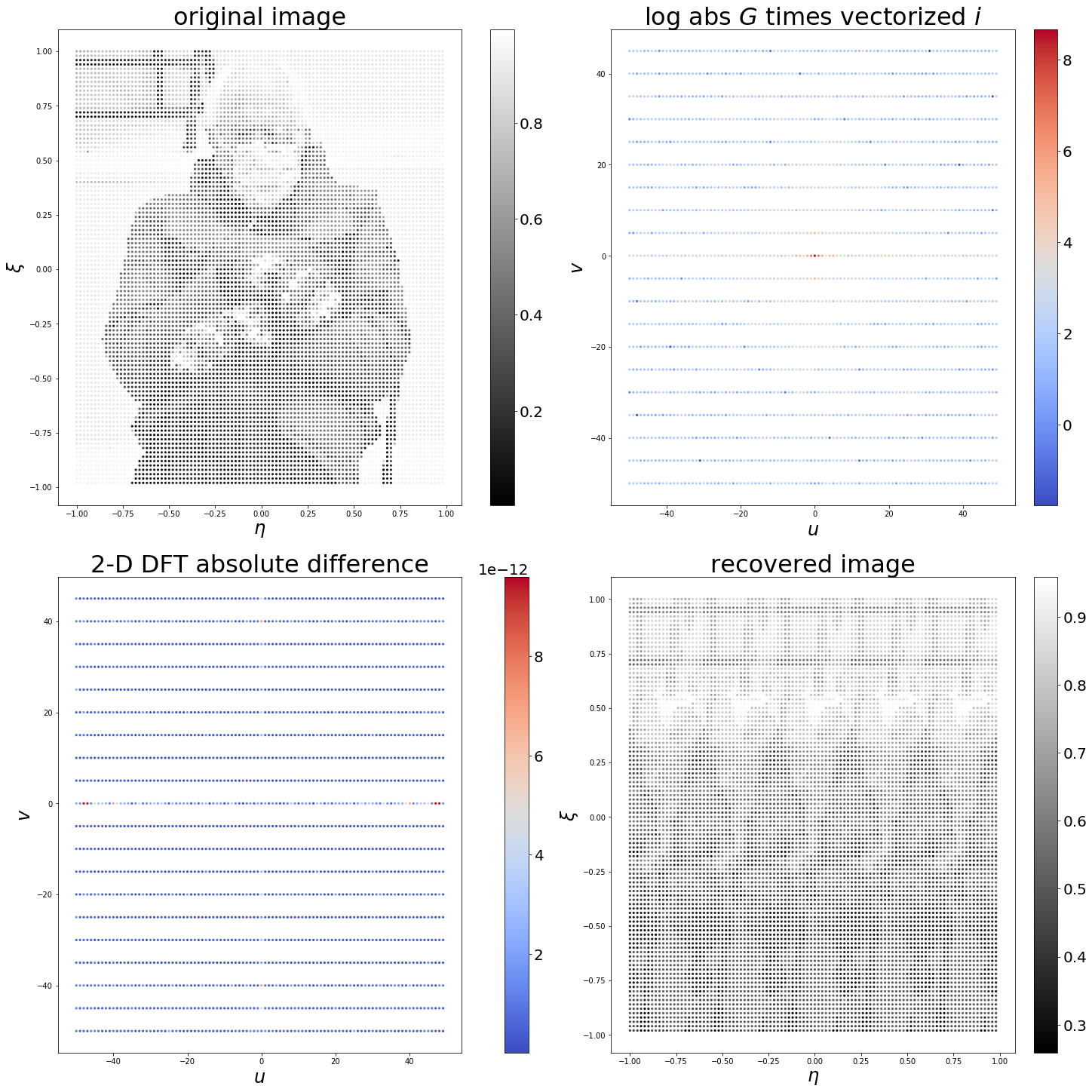
With an image of even size, the results are similar:

Image shape 100x100 Ngrid 10000
Rectangular frame, 51x51. Number of baselines (if no cuts introduced): 10201
Number of baselines (after cuts): 10000
Mean 2-D DFT error: 3.3816143014168846e-13

/assets/output_DFT_comp_nofolding100.svg

Same as above, but for a $100\times 100$ image, rather than $99\times 99$.

With the square frame antenna array with antennas regularly spaced at distance of 0.5 wavelengths, the $\bm{G}$ matrix—with factors of (-1) added, only one conjugate visibility pair for each baseline (rather than antenna pair) used in its construction, and with one member removed of each conjugate pair of the maximum baseline observed along each direction along which the image we wish to recover must be of even size—indeed matches the tensor product of two DFT matrices and performs the 2-D DFT when applied to a vectorized brightness temperature image to produce a vectorized vector of visibilities.

Do we really need all those rows? (Conjugate visibility pairs keep it [the recovered sky brightness image] real)

From our perspective, we have included redundant information, as we have two rows of $\bm{G}$ for each baseline pair, but only one correlator output. Another way of saying this is that we know the temperature map is real and thus its Fourier transform is conjugate symmetric, so rather than writing our recovery problem as constrained

\[\widehat{t} = \underset{t\in\mathbb{C}^{N_{vis}'}}{\arg\min} || \bm{G}'t - v' ||_2^2 \text{ subject to } t\in\mathbb{R}^{N_{vis}'}\]

where $\bm{G}'$ has one row and correspondingly $v'$ one element per distinct baseline (i.e., one row for each set $\{(a,b),\, (-a,-b)\}$) and where $N_{vis}' = 2N_xN_y-N_x-N_y+1 = \frac{N_{vis}-1}{2}+1$ for a rectangular $N_x \times N_y$ antenna array, we constrain $t$ to assume real values by hard-coding conjugate symmetry in its Fourier transform $v$, doubling its length. Indeed, if we drop the double observation of each nonzero baseline, the recovered temperature map may have substantial energy in the imaginary part.

## HELPER FUNCTION ##

def delete_redundant(G, v, us, vs):
    # for every baseline pair not on the v-axis, delete the baseline with negative u
    # for every baseline pair on the v-axis, delete the one with negative v value
    # keep the baseline (0,0) as it's only observed once
    toss = np.logical_or(us < 0, np.logical_and(us == 0, vs < 0))
    keep = np.logical_not(toss)
    return G[keep,:], v[keep], us[keep], vs[keep] 

## GET "UNCONSTRAINED" IMAGE BY DELETING VISIBILITIES AT "REAL-SIGNAL REDUNDANT" BASELINES ##

G, v, _, _ = delete_redundant(G, v, us, vs)
irec = (np.linalg.pinv(G) @ v).reshape((M,N))

## PLOT "UNCONSTRAINED" TEMPERATURE MAP ##

fig, (ax1,ax2,ax3) = plt.subplots(1,3, figsize=(15,5), constrained_layout=True)
im1 = ax1.imshow(np.real(irec), cmap='coolwarm', vmin=-1, vmax=1)
ax1.axis('off')
ax1.set_title("real part", fontsize=24)
im2 = ax2.imshow(np.imag(irec), cmap='coolwarm', vmin=-1, vmax=1)
ax2.axis('off')
ax2.set_title("imaginary part", fontsize=24)
im3 = ax3.imshow(np.abs(irec), cmap='coolwarm', vmin=-1, vmax=1)
ax3.axis('off')
ax3.set_title("modulus", fontsize=24)
fig.subplots_adjust(right=0.85)
cbar_ax = fig.add_axes([0.87, 0.18, 0.01, 0.645])
fig.colorbar(im2, cax=cbar_ax)
plt.savefig('complex-part.svg', bbox_inches='tight')

## NORM COMPARISON WITH ORIGINAL TEMPERATURE MAP ##

print(f"Loss, unconstrained temperature map: {np.linalg.norm(G@irec.flatten() - v)}")
print(f"Mean absolute value of real part: {np.mean(np.abs(np.real(irec)))}")
print(f"Mean absolute value of imaginary part: {np.mean(np.abs(np.imag(irec)))}")
print(f"Condition number of G: {np.linalg.cond(G)}")

Loss, unconstrained temperature map: 1.897639874056643e-11
Mean absolute value of real part: 0.41270865498934917
Mean absolute value of imaginary part: 0.12383688546215746
Condition number of G: 1.0000000000000053

Deleting rows of $\bm{G}$ does not change its conditioning because $\bm{G}$ is a unitary matrix (if we scale it by $\frac{1}{\sqrt{MN}}$). If we delete $0\leq k < MN$ rows from $\bm{G}$ to form $\bm{G}'$, the remaining rows will still be orthonormal vectors in $\mathbb{C}^{MN}$ but will no longer form a basis. Consequently, $\bm{G}'^*$, the Hermitian transpose of $\bm{G}'$, is a right-inverse of $\bm{G}'$:

\[\bm{G}'\bm{G}'^* = \mathbf{I}_{MN-k},\]

where $k$ is the number of excised rows. In other words, if $\mathbf{U\Sigma V}^*$ is a singular-value decomposition of $\bm{G}'$, then $\bm{G}'\bm{G}'^* = \mathbf{U\Sigma\Sigma}^*\mathbf{U}^* = \mathbf{I} (= \mathbf{U}^*\mathbf{U})$, and thus all singular values of $\bm{G}'$ are unimodular (or, have modulus 1 to numerical precision). In fact, they are unchanged from $\bm{G}$ and exactly 1.

We see that $\texttt{pinv}$ finds a solution with norm of zero (to the precision we could reasonably expect, given the DFT error). However, unlike the true zero-norm solution—the real brightness temperature map we used for the simulation—the solution $\texttt{pinv}$ settles on is substantially nonreal.

From left: the real part, imaginary part, and magnitude of the brightness temperature map recovered when just one visibility from each antenna pair (corresponding to a distinct baseline) is used. Since the brightness temperature map's DFT is no longer constrained to be conjugate-symmetric, the recovered brightness temperature map is free to adopt complex values).

A "DFT scenario" therefore requires both observations of the visibilities associated with antenna pair chosen to represent each baseline, even though in practice there is but one correlator output. To this visibility reading at the correlator output we can add its complex conjugate to enforce realness in the recovered brightness temperature image.

Do we really need all those columns? (Or: why we need to recover the brightness temperature at direction cosines that don't actually exist)

The corner pseudo-directions—the pixels of brightness temperature 0 we attempt to recover associated with direction cosine pair $(\xi, \eta)$ whose 2-norm is greater than 1—do much to stabilize the $\bm{G}$ matrix. Without their inclusion, the corresponding $\bm{G}$ matrix (still using regularly spaced direction cosines!) can be poorly conditioned.

def get_G_matrix_corners(baselines, xis, etas, corners=True):
    Ngrid = len(xis)*len(etas) # number of cosine directions
    Nvis = len(baselines) # number of baselines

    xis, etas = np.meshgrid(xis, etas, indexing='ij')
    if corners == False:
        visible_mask = xis**2 + etas**2 <= 1
        xis = xis[visible_mask]
        etas = etas[visible_mask]
        Ngrid = len(xis)
    xis = np.outer(np.ones((Nvis,)), xis.flatten())
    etas = np.outer(np.ones((Nvis,)), etas.flatten())
    us, vs = baselines[:,0], baselines[:,1]
    us = np.outer(us, np.ones((Ngrid,)))
    vs = np.outer(vs, np.ones((Ngrid,)))
    factor = (-1)**(np.round(2*(us + vs))%2)
    return factor*np.exp(-2*np.pi*1j*(us*xis+ vs*etas))


for Nx, Ny in zip([17,33,65,129], [17,33,65,129]):
    M = 2*Nx+1
    N = 2*Ny+1
    du, dv = 0.5, 0.5
    cond = {}
    for t in [1,2,4,8]:
        points_spatial = make_rectangle(Nx,Ny,du,dv,t=t)
        baselines = get_baselines(points_spatial, redundant_baselines=False)

        dxi = 2/M
        deta = 2/N
        xis = -1+np.arange(M)*dxi
        etas = -1+np.arange(N)*deta

        G = get_G_matrix_corners(baselines, xis, etas, corners=False)

        cond[(Nx,Ny,t)] = np.linalg.cond(G)

Let's examine the contents of the dictionary $\texttt{cond}$ in tabular form:

Nx/Ny	t=1	t=2	t=4	t=8	t=16	t=32
9	1.217e+16	2.391e+15	4.407	not computed	not computed	not computed
17	4.130e+15	1.699e+15	5.941	5.644	not computed	not computed
33	1.605e+15	1.339e+15	5.368e+14	8.561	8.127	not computed
65	6.633e+14	1.437e+15	8.011e+14	12.54	12.35	12.16

Each data cell gives the condition number of the $\bm{G}$ matrix associated with the corresponding configuration. The number of antennas along each bar ($N_x=N_y$, so the number of antennas, before decimation, is the same along the the $u$-axis and $v$-axis) is given by the value in each row's first column. In the second column ($t=1$), we have no the results of experiments without decimation, so antenna spacing is always half a wavelength. In the third column, $t=2$, so every other antenna along the horizontal (along-track) bars is removed; the total number of antennas along the horizontal bars becomes $(N_y+1)/2$ and their spacing along these bars 1 wavelength. Moving along a row, in each successive column, we leave the vertical, across-track ($u$-axis) bars untouched and delete every other remaining antenna on the horizontal, along-track ($v$-axis) bars of our square frame antenna array.

Recall that, when we include the corner direction cosines, $\bm{G}$ is (proportional to) unitary, and the deletion of its rows (by including fewer visibility samples in our inversion) does not affect its condition number (it remains one). When we don't try to recover the (zero) brightness temperature at these corner direction cosines, the condition number of $\bm{G}$ can be near the inverse of the numerical precision error, and a partial recovery help stabilize $\bm{G}$ by removing highly correlated rows. When working in these coordinates with a regular array, at least, we need to keep the corners at 0 K brightness temperature. (Once again, college radio dispenses bad advice.)

Deviations from the DFT: deleting rows or columns of $\bm{G}$

Folding due to undersampling of the visibilities

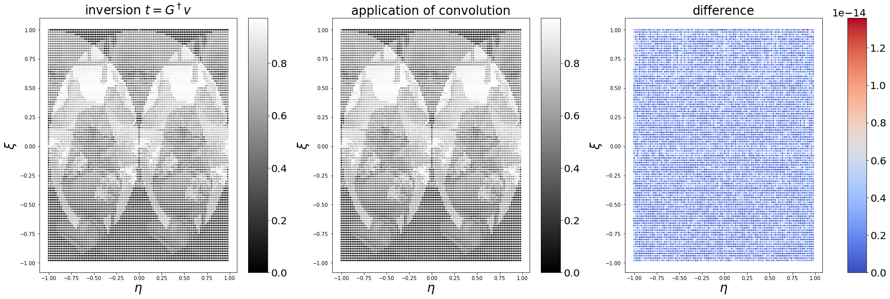
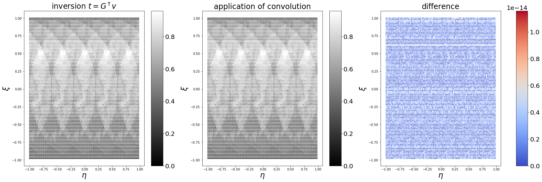
The recovered brightness temperature image $i_{rec} = \bm{G}^\dagger \bm{G} i$ will differ from $i$ if the visibilities $\bm{G} i$ sample the $u$-$v$ plane insufficiently richly. This can happen if our antenna layout diverges from that of the DFT scenario detailed above or if we choose to invert $\bm{G}$ in stages. We consider a particular form of the former situation, where there is regular structure in the missing antennas on the frame.

Lemma: folding and decimation are transform pairs

An elementary property of the DFT—though one that is often omitted from transform tables—is that decimation in the frequency domain corresponds to folding in the time domain (and vice versa). In the following discussion, we continue our convention of using the $\texttt{np.fft}$ normalization coefficient convention: normalization of $1$ for the $M$-point DFT and $\frac{1}{M}$ for the $M$-point inverse DFT.

Lemma 1 Let $x$ be an $M$-point discrete signal and $X$ its $M$-point DFT. Suppose $s$ divides $M$. Consider the $\frac{M}{s}$-point discrete signal $x_f$ whose DFT is $X$, decimated by the factor $s$: for each $\omega\in\mathbb{Z}/\frac{M}{s}\mathbb{Z}$, $X_f[\omega] = X[s\omega]$. We may write $x_f$ as follows:

\[x_f[n] = x[n] + x\left[n+\frac{M}{s}\right] + \ldots + x\left[n+(s-1)\frac{M}{s}\right]\]

for each $n\in\mathbb{Z}/\frac{M}{s}\mathbb{Z}.$

Proof. Using the $M$-point DFT, we can express the samples of $X$ that are included in the $\frac{M}{s}$-point signal $X_f$ as follows:

\[\begin{aligned} X_f[n] = X[sn] &= \sum_{k=0}^{M-1}x[k]e^{-2\pi i (sn)k/M}\\ &= \sum_{k=0}^{M-1}x[k]e^{-2\pi i k/(M/s)}\\ &= \sum_{k=0}^{\frac{M}{s}-1} x[k]e^{-2\pi i kn/(M/s)} + \sum_{k=\frac{M}{s}}^{2\frac{M}{s}-1} x[k]e^{-2\pi i kn/(M/s)} +\ldots + \sum_{k=(s-1)\frac{M}{s}}^{M-1} x[k]e^{-2\pi i kn/(M/s)}\\ &= \sum_{k=0}^{\frac{M}{s}-1} x[k]e^{-2\pi i kn/(M/s)} + \underbrace{e^{-2\pi i n \left(\frac{M}{s}\right)/\left(\frac{M}{s}\right)}}_{1}\sum_{k=0}^{\frac{M}{s}-1} x\left[k+\frac{M}{s}\right]e^{-2\pi i kn/(M/s)}+\ldots \\&\quad + \underbrace{e^{-2\pi i n (s-1)\left(\frac{M}{s}\right)/\left(\frac{M}{s}\right)}}_{1}\sum_{k=0}^{\frac{M}{s}-1} x\left[k+(s-1)\frac{M}{s}\right]e^{-2\pi i kn/(M/s)}\\ &= \sum_{k=0}^{\frac{M}{s}-1}\left(x[k] + x\left[k+\frac{M}{s}\right] + \ldots + x\left[k+(s-1)\frac{M}{s}\right]\right)e^{-2\pi i kn/(M/s)}. \end{aligned}\]

In the third line of (19), we broke up the $M$-point DFT sum into $s$ distinct $\frac{M}{s}$-point DFT sums and then brought them under a single $\frac{M}{s}$-point DFT summand.

Since this DFT expansion holds for all $n\in\mathbb{Z}/\frac{M}{s}$, the signal $x_f$ is therefore the $\frac{M}{s}$-periodic sum given in equation (18) of the lemma.□

Depending on how we normalize $\bm{G}$, we may need to scale our expression above by $\frac{1}{s}$. We can interpret $\bm{G}$ as performing $\frac{MN}{s}$ distinct 2-D DFTs that are $M$-point along one axis and $N$-point along the other, and $\bm{G}^\dagger$ as performing an inverse 2-D DFT that is $M$-point along one axis and $\frac{N}{s}$-point along the other; this

Treating each row as a one-dimensional signal and decimating its $M$-point, 1-D DFT by a factor of $s=2$ is equivalent to removing one antenna out of every two along our horizontal arm.

Folding by undersampling along the $v$-axis

We start by removing one antenna out of two along the $v$-axis.

Nx, Ny = 100, 100
du, dv = 0.5, 0.5
t=2
points_spatial = make_rectangle(Nx,Ny,du,dv,t=t)
baselines = get_baselines(points_spatial, redundant_baselines=False)

At left, the antenna positions in the decimated ($t=2$) scenario. At right, the corresponding visibility sample locations (baselines).

The aliasing we observe in the image recovered from the undersampled visibilities takes the form of highly structured folding consistent with Lemma 1.

dxi = 2/M
deta = 2/N
xis = -1+np.arange(M)*dxi
etas = -1+np.arange(N)*deta

G = get_G_matrix(baselines, xis, etas)
i = I.flatten()
v = G @ i

# THE PLOTTING AND THE COMPARISON ##
xis, etas = np.meshgrid(xis, etas, indexing='ij')
freqx, freqy = 2*baselines[:,0], 2*baselines[:,1]


fft_direct = np.fft.fft2(I).flatten()

fig, ((ax1,ax2),(ax3,ax4)) = plt.subplots(2,2, figsize=(20,20), constrained_layout=True)


# plot the original image
im1 = ax1.scatter(etas.flatten(), -xis.flatten(), c=i, marker='.', s=18, cmap='gray')
ax1.set_title('original image',fontsize=32)
ax1.set_xlabel(r'$\eta$', fontsize=24)
ax1.set_ylabel(r'$\xi$', fontsize=24)

us, vs = np.meshgrid(np.arange(M, dtype=int), np.arange(N, dtype=int), indexing='ij')
us, vs = np.where(us >= M//2, us-M, us).flatten(), np.where(vs >= N//2, vs-N, vs).flatten()

# plot the 2-D DFT computed using G
im2 = ax2.scatter(freqx, freqy, c=np.log(np.abs(v)), marker='.', s=18, cmap='coolwarm')
ax2.set_title(r'log abs $G$ times vectorized $i$', fontsize=32)
ax2.set_xlabel(r"$u$", fontsize=24)
ax2.set_ylabel(r"$v$", fontsize=24)

freq1 = dict([((fx,fy),val) for fx,fy,val in zip(freqx,freqy,v) if fx!=50])
freq2 = dict([((fx,fy),val) for fx,fy,val in zip(us, vs, fft_direct)])

diff = [np.abs(freq1[k] - freq2[k]) for k in freq1.keys()]

# plot the comparison
im3 = ax3.scatter(list(map(lambda x:x[0], freq1.keys())), list(map(lambda x:x[1], freq1.keys())), c=diff, marker='.', s=18, cmap='coolwarm')
ax3.set_title('2-D DFT absolute difference', fontsize=32)
ax3.set_xlabel(r"$u$", fontsize=24)
ax3.set_ylabel(r"$v$", fontsize=24)

# plot the (folded) recovered image
recovered = np.real(np.linalg.pinv(G)@v) ## <-- THE RECOVERED IMAGE FROM THE VISIBILITIES G@i USING THE PSEUDO-INVERSE OF G
im4 = ax4.scatter(etas.flatten(), -xis.flatten(), c=recovered, marker='.', s=18, cmap='gray')
ax4.set_title('recovered image', fontsize=32)
ax4.set_xlabel(r"$\eta$", fontsize=24)
ax4.set_ylabel(r"$\xi$", fontsize=24)

c1 = fig.colorbar(im1, ax=ax1)
c1.ax.tick_params(labelsize=20)
c2 = fig.colorbar(im2, ax=ax2)
c2.ax.tick_params(labelsize=20)
c3 = fig.colorbar(im3, ax=ax3)
c3.ax.tick_params(labelsize=20)
c3.ax.yaxis.get_offset_text().set_fontsize(20)
c4 = fig.colorbar(im4, ax=ax4)
c4.ax.tick_params(labelsize=20)
plt.show()
plt.savefig(f'output_DFT_comp_folded_{t}.svg', bbox_inches='tight')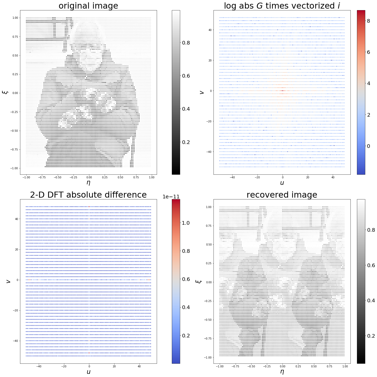

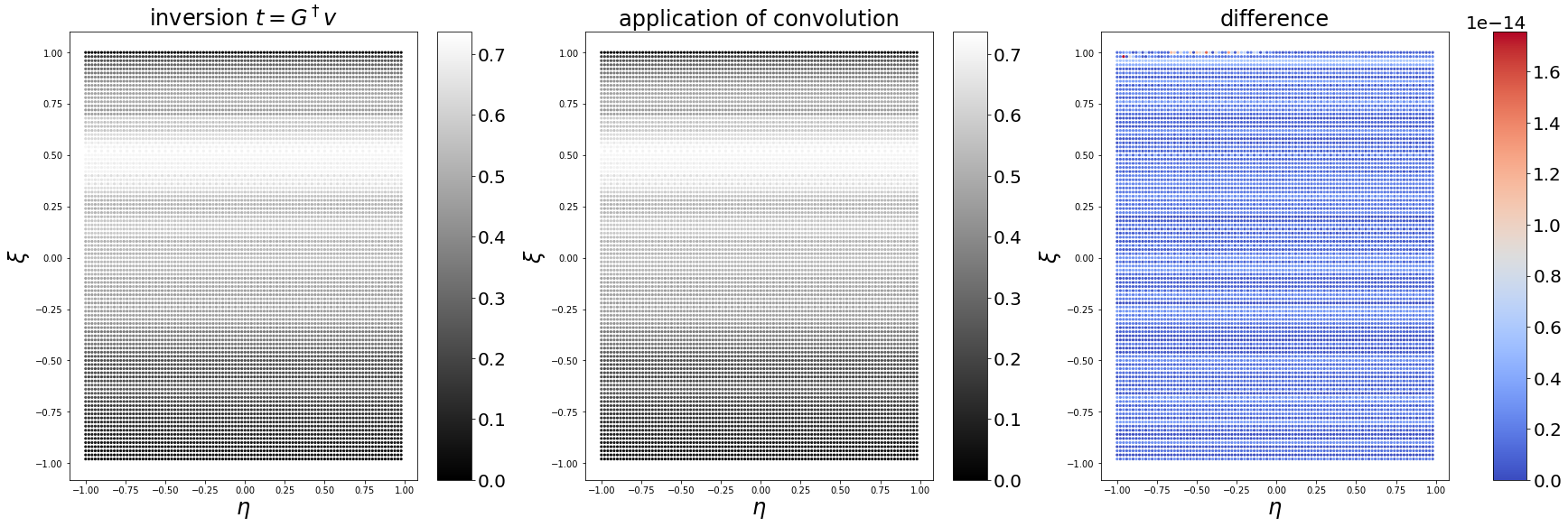
Clockwise, from top left: The original image; the visibility samples obtained by multiplying the vectorized image by $\bm{G}$ (with rows associated with the $t=2$ decimation scenario); the absolute difference between these visibility samples and the ordinary 2-D DFT where we have samples to compare (one column out of two along the $v$-axis); the image $\bm{G}^\dagger\bm{G}i$ recovered from the undersampled visibilities ($\bm{G}$ encodes the missing visibilities with missing rows).

Continuing in this manner, we keep one antenna out of five and observe five-way folding.

Nx, Ny = 100, 100
du, dv = 0.5, 0.5
t=5
points_spatial = make_rectangle(Nx,Ny,du,dv,t=t)
baselines = get_baselines(points_spatial, redundant_baselines=False)

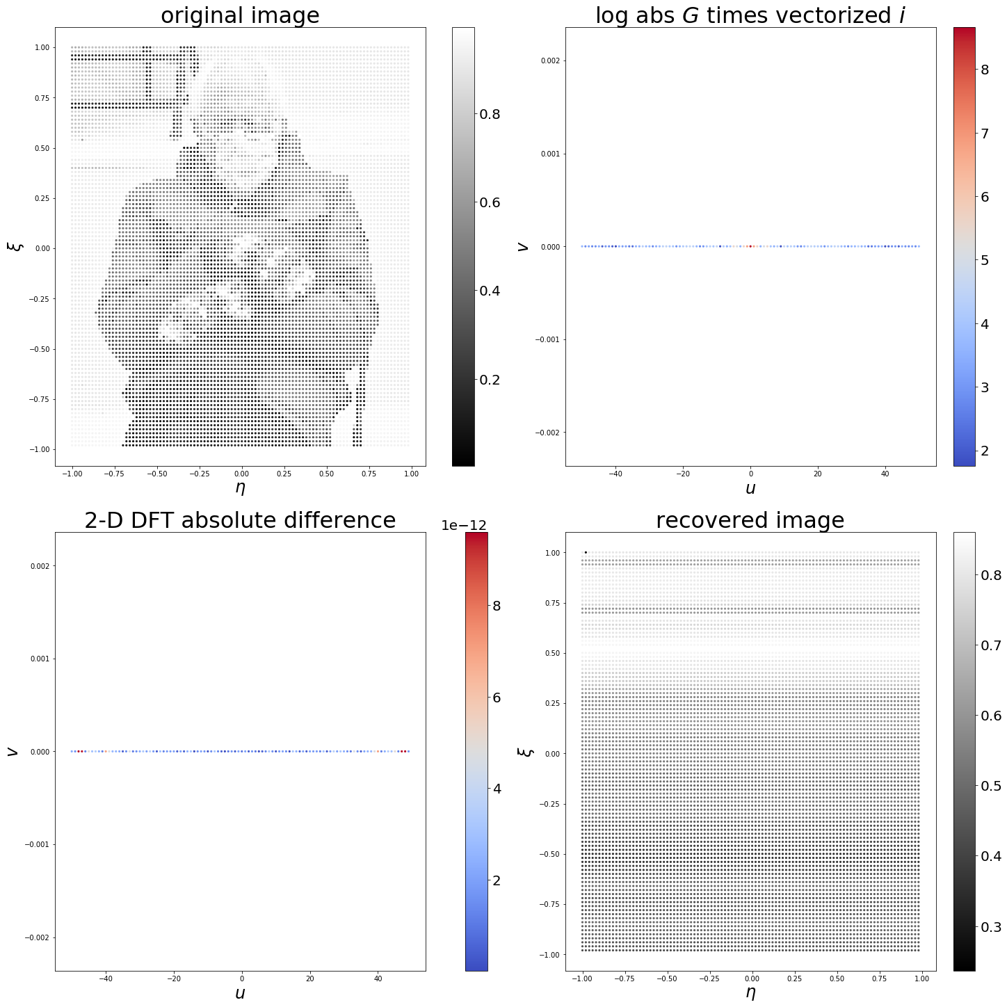
At left, the antenna positions in the decimated ($t=5$) scenario. At right, the corresponding visibility sample locations (baselines).

Clockwise, from top left: The original image; the visibilities sampled by our antenna layout, decimated along the $v$-axis by a factor of 5; the absolute difference between these visibility samples and the ordinary 2-D DFT where we have samples to compare; the image recovered from the undersampled visibilities.

Ultimately, if we decimate all in the $v$-direction, so that the rectangular frame has antennas on just a single vertical bar and every sampled visibility has no $v$-component, the image recovered will include only the DC components of each row.

Same as above, but if we replace our square frame with a single arm. With just one $v$ value sampled, in the image plane, we get the DC value repeated for each $\xi$ repeated across the $\eta$.

We compare a direct application of the folding mechanism in equation (18) with the folding produced by this structured undersampling of the $u$-$v$ plane by removing 1 out of $t$ antennas along the horizontal bars.

At top, the (reshaped) image $\bm{G}^\dagger \bm{G} i$, where $\bm{G}$ is associated with a DFT after decimating the antennas on the square frame by a factor of 2 in the along-track $v$-direction (only one column is kept out of 2, resulting in a folded image along-track). In the middle, the error image recovered from the convolution given by our folding model in (18). At the bottom, the error between these two images. The difference between the recovered images is negligible.

The same as above, but with $t=5$.

The same as above, but with $t=50$.

Another form of row removal: partial recovery

Even if we have sufficient visibility samples, we may wish to invert only a subset for computational resource constraints or stability concerns.

If the rows of $\bm{G}$ are orthogonal, this works out especially nicely (though if the rows of $\bm{G}$ are orthogonal, we wouldn't, of course, encounter any trouble (pseudo-)inverting a $\bm{G}$ matrix due to poor conditioning). If we partition the rows of $\bm{G}$ into two distinct sets, placing the $N_1$ rows of the former set in $\bm{G}_1$ and the $N_2$ rows of the latter in $\bm{G}_2$, we can recover $\bm{G}^\dagger \bm{G}i$ simply by summing $\bm{G}_1^\dagger\bm{G}_1i$ and $\bm{G}_2^\dagger\bm{G}_2i$. This works because $\bm{G}_1^\dagger$ maps visibilities into the orthogonal complement of the null space of $\bm{G}_1$, which is precisely the null space of $\bm{G}_2$, and vice versa.

\[\begin{aligned}\widehat{i} = \bm{G}^\dagger v &= \underset{i \in \mathbb{C}^{N_{vis}}}{\arg\min} ||\bm{G}i - v||_2^2\\ &= \underset{i \in \mathbb{C}^{N_{vis}}}{\arg\min} ||(\bm{G}_1 i- v_1) + (\bm{G}_2i-v_2)||_2^2 && \text{(disjointness of rows in partition)}\\ &= \underset{i \in \mathbb{C}^{N_{vis}}}{\arg\min} ||\bm{G}_1 i- v_1||_2^2 + ||\bm{G}_2i-v_2||_2^2 && \text{(Pythagorean theorem)}\\ &= \underset{i_1 \in \mathbb{C}^{N_1}}{\arg\min} ||\bm{G}_1i-v_1||_2^2 + \underset{i_2 \in \mathbb{C}^{N_2}}{\arg\min} ||\bm{G}_2i-v_2||_2^2 &&\text{(orthogonality of the rows of $\bm{G}$)}\\ &= \bm{G}_1^\dagger v_1 + \bm{G}_2^\dagger v_2 \end{aligned}\]

The separation of the terms in the fourth row of (20) works because $\mathbb{C}^{N_{vis}} = \text{null}\,\bm{G}_1 \oplus \text{null}\,\bm{G}_2$, and consequently $i$ can be decomposed via orthogonal projection as $i=i_{\text{null}\, \bm{G}_1} + i_{\text{null}\, \bm{G}_2}$. The solution to the first empirical risk term lies in the orthogonal complement of the null space of $\bm{G}_1$–-that is, in the null space of $\bm{G}_2$–-and the solution to the second lies in the null space of $\bm{G}_1$. We can therefore choose the component $i_{\text{null}\,\bm{G}_2}$ to minimize the energy in the first term and choose the component $i_{\text{null}\,\bm{G}_1}$ to minimize the energy in the second, and sum the results.

Indeed, an elementary matrix calculation shows that, if the $M\times N$ matrix $\bm{G}$ is invertible and its rows are orthogonal over $\mathbb{C}^N$, no matter how we partition the rows into $\bm{G}_1$ and $\bm{G}_2$, we have that

\[\begin{aligned} I &= \bm{G}^* \left(\bm{G}^{*}\right)^{-1} \bm{G}^{-1}\bm{G}\\ &= \begin{pmatrix} \bm{G}_1^* & \bm{G}_2^* \end{pmatrix} \begin{pmatrix} \bm{G}_1^* & \bm{G}_2^* \end{pmatrix}^{-1} \begin{pmatrix} \bm{G}_1 \\ \bm{G}_2 \end{pmatrix}^{-1} \begin{pmatrix}\bm{G}_1 \\ \bm{G}_2 \end{pmatrix}\\ &= \begin{pmatrix}\bm{G}_1^* & \bm{G}_2^*\end{pmatrix}\left(\begin{pmatrix}\bm{G}_1\\\bm{G}_2\end{pmatrix}\begin{pmatrix}\bm{G}_1^* & \bm{G}_2^*\end{pmatrix}\right)^{-1}\begin{pmatrix}\bm{G}_1\\ \bm{G}_2\end{pmatrix}\\ &=\begin{pmatrix}\bm{G}_1^* & \bm{G}_2^*\end{pmatrix} \begin{pmatrix}\bm{G}_1\bm{G}_1^* & \bm{G}_1\bm{G}_2^*\\ \bm{G}_2\bm{G}_1^* & \bm{G}_2\bm{G}_2^*\end{pmatrix}^{-1}\begin{pmatrix}\bm{G}_1\\ \bm{G}_2\end{pmatrix}\\ &= \begin{pmatrix}\bm{G}_1^* & \bm{G}_2^*\end{pmatrix} \begin{pmatrix}\bm{G}_1\bm{G}_1^* & \mathbf{0}\\ \mathbf{0} & \bm{G}_2\bm{G}_2^*\end{pmatrix}^{-1}\begin{pmatrix}\bm{G}_1\\ \bm{G}_2\end{pmatrix}\\ &= \bm{G}_1^*\left(\bm{G}_1\bm{G}_1^*\right)^{-1}\bm{G}_1 + \bm{G}_2^*\left(\bm{G}_2\bm{G}_2^*\right)^{-1}\bm{G}_2\\ &= \bm{G}_1^\dagger\bm{G}_1 + \bm{G}_2^\dagger\bm{G}_2, \end{aligned}\]

so long as $\bm{G}$ is partitioned into $\bm{G}_1$ and $\bm{G}_2$ such that the rows of $\bm{G}_1$ are orthogonal to the rows of $\bm{G}_2$: that is, $\bm{G}_i\bm{G}_{3-i}^* = \mathbf{0}$ for $i=1,2$. Thus, we can recover the image $i$ with separate inversion of $\bm{G}_1$ and $\bm{G}_2$:

\[i = \bm{G}_1^\dagger \bm{G}_1 i + \bm{G}_2^\dagger \bm{G}_2 i = \bm{G}_1^\dagger v_1 + \bm{G}_2^\dagger v_2.\]

Since the matrices $\bm{G}_1$ and $\bm{G}_2$ are "short," with linearly independent rows but linearly dependent columns, $\bm{G}_i\bm{G}_i^*$ is invertible and the Moore-Penrose pseudoinverse of $\bm{G}_i$ is a right inverse that can be written, for $i=1,2,$ as $\bm{G}_i^\dagger = \bm{G}_i^*(\bm{G}_i\bm{G}_i^*)^{-1}$.

If the cross terms $\bm{G}_{i}\bm{G}_{3-i}^* \neq \mathbf{0}$, the central matrix in (21) is no longer block diagonal (though in certain cases it may be useful to recognize that the diagonal terms remain invertible). We can use the pseudoinverse formula for a row-partitioned matrix (see Baksalary and Baksalary (2007)):

\[ G^\dagger = \begin{pmatrix}\left(\bm{G}_1P_{\text{null}\,\bm{G}_2}\right)^\dagger & \left(\bm{G}_2P_{\text{null}\,\bm{G}_1}\right)^\dagger \end{pmatrix}, \]

where for $i=1,2,$ we use the "independent rows" formula for the Moore-Penrose pseudoinverse to write

\[P_{\text{null}\,\bm{G}_i} = \mathbf{I} - \bm{G}_i^*\left(\bm{G}_i\bm{G}_i^*\right)^{-1}\bm{G}_i = \mathbf{I}-\bm{G}_i^\dagger\bm{G}_i.\]

In this case, we not only have to pseudoinvert $\bm{G}_1$ and $\bm{G}_2$ we need also pseudoinvert the two cross terms $\bm{G}_i - \bm{G}_i\bm{G}_{3-i}^\dagger\bm{G}_{3-1}$ for $i=1,2.$ (For instance, ife we separate a "quincunx" baseline pattern into two overlapping DFT—or, more precisely, perfectly conditioned—grids for the $\bm{G}_1$ and $\bm{G}_2$, it is the cross-terms that introduce instability.)

The regressionheads out there (that is, social scientists and other multivariate least-squares regression practitioners) are very familiar with the failure of equation (22) to apply when rows of $\bm{G}_1$ are correlated to rows of $\bm{G}_2$—at least if they tilt their heads. For instance, attempting to recover a "low-frequency component" image $i_i$ from $v_1 = \bm{G}_1 i$ without the orthogonality condition that the rows of $\bm{G}_1$ (the observation model for the "low-frequency visibilities") be orthogonal to the rows of $\bm{G}_2$ (the observation model for the "high-frequency visibilities") is essentially the transpose of the omitted-variables bias in econometrics in which the matrix we are seeking to pseudoinvert is missing columns (omitted variables) that are correlated to the observed columns. As a result, a pseudoinverse will learn incorrect weights as it attributes the outcome only to observed variables. We more directly encounter the omitted-variables bias in our choice of the sampling of our sky brightness image: each pixel removed affects how much brightness temperature the other pixels contribute to produce the visibility image (if we hold the visibilities fixed). Choosing as our inversion approach the (possibly regularized) Moore-Penrose pseudoinverse of a Riemann sum operator (i.e., a sort of least-squares empirical risk minimization) constrains how our recovered brightness temperature image can evolve over direction cosines.

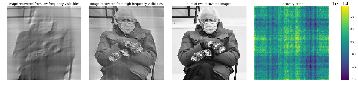
We presently demonstrate this technique of row-partitioning, at least in an "easy mode." In this experiment, we place the rows into two categories: those associated with "low-frequency" visibilities and those associated with "high-frequency" visibilities. Since we have a DFT scenario, the rows of $\bm{G}$ are all orthogonal, so no matter how we partition them into $\bm{G}_1$ and $\bm{G}_2$, we know that each row in $\bm{G}_1$ will be orthogonal each row in $\bm{G}_2$.

## READ IMAGE AND DEFINE DFT SCENARIO ##

I = mpimg.imread('bernie.jpg')
M, N = I.shape
Nx = M//2+1
Ny = N//2+1
dx, dy = 0.5, 0.5
points_spatial = make_rectangle(Nx, Ny, dx, dy)
baselines = get_baselines(points_spatial, redundant_baselines=False) 
maxu, maxv = np.max(baselines, axis=0)
if M % 2 == 0:
    baselines = baselines[baselines[:,0] < maxu]
if N % 2 == 0:
    baselines = baselines[baselines[:,1] < maxv]

## PARTITION THE G MATRIX INTO TWO SETS, BASED ON L1 BASELINE NORM ##

f_c = Nx//2 # cutoff frequency
us, vs = baselines[:,0], baselines[:,1]

# square cutoff (distance from origin, using the Manhattan pedestrian or cyclist metric [the climate crisis obliges us])
lf_rows = np.abs(us) + np.abs(vs) <= f_c # rows of G, v corresponding to "low-frequency baselines"
hf_rows = np.abs(us) + np.abs(vs) > f_c # rows of "high-frequency baselines"
Glf = G[lf_rows,:]
Ghf = G[hf_rows,:]

image_lf = np.linalg.pinv(Glf)@Glf@i
image_hf = np.linalg.pinv(Ghf)@Ghf@i
image_total = image_lf + image_hf

fig, (ax1,ax2,ax3,ax4) = plt.subplots(1,4, figsize=(20,5), constrained_layout=True)

    
img1 = ax1.imshow(np.real(image_lf).reshape((Nx,Ny)))
ax1.axis('off')
ax1.set_title("Image recovered from low-frequency visibilities")

img2 = ax2.imshow(np.real(image_hf).reshape((Nx,Ny)))
ax2.axis('off')
ax2.set_title("Image recovered from high-frequency visibilities")

img3 = ax3.imshow(np.real(image_sum).reshape((Nx,Ny)))
ax3.axis('off')
ax3.set_title("Sum of two recovered images")

img4 = ax4.imshow((np.real(image_sum) - I).reshape((Nx,Ny)))
c4 = fig.colorbar(img4, aspect=40, shrink=0.85)
c4.ax.yaxis.get_offset_text().set_fontsize(20)
ax4.axis('off')
ax4.set_title("Recovery error")

The two images are indeed the corresponding low-frequency and high-frequency components, though contain artifacts due to the implicit windowing and periodization. The fused image is what we expect to recover.

Other deviations from the DFT

In the DFT scenario, the $\bm{G}$ matrix is (if scaled properly) unitary because the $e^{-2\pi i(u\xi + v\eta)}$ term, as it evolves across the $(\xi, \eta)$ brightness temperature pixels for a fixed $(u,v)$ baseline (across the row of $\bm{G}$) or across the baselines for a fixed brightness temperature pixel (across a column of $\bm{G}$), produces orthogonal vectors. If we make either sampling of the brightness temperature map irregular (by attempting to recover an image whose pixels are irregularly sampled in satellite-centered direction cosines $(\xi, \eta)$) or sampling of the baselines $(u,v)$ irregular (by using an irregular antenna array), we may produce a $\bm{G}$ matrix that is poorly conditioned.

The $\xi$-$\eta$ plane is not the most convenient one for locating points on Earth (it corresponds to the projection of the celestial sphere onto the tangent plane along the $w$-axis (nadir), and is not invariant as the satellite moves). Uniform sampling in coordinate systems convenient for locating points on Earth—such as latitude and longitude relative to the subsatellite point—are highly nonuniform in $\xi$-$\eta$ coordinates.

Moreover, configurations that generate a regular grid of baseline samples will sample the $u$-$v$ plane inefficiently; that is, certain baselines will necessarily be sampled many times if a regular DFT grid is to be filled out. Redundant observations need not be thrown out, as they were in this exercise, as they can help denoise the image. But those redundant observations limit the resolution of the sky brightness map recovered by the inversion. Consequently, we may wish to sample the $u$-$v$ plane irregularly to maximize the number of distinct baselines sampled and thus the resolution of the image after inversion of the $\bm{G}$ matrix. Unfortunately, irregular sampling of the $u$-$v$ plane can greatly affect the conditioning of the $\bm{G}$ matrix; the unitarity of the $\bm{G}$ matrix in the DFT smapling scenario is enabled only by the sampling of regular, orthogonal visibility frequencies in the $u$-$v$ plane. Irregular sampling can lead to highly correlated rows of the $\bm{G}$ matrix and thereby complicate the inversion process.

References

A. Richard Thompson, James M. Moran, and George W. Swenson Jr. Inteferometry and Synthesis in Radio Astronomy, Third Edition (open access download link). The standard introductory radio astronomy text.
Jerzy K. Baksalary, Oskar Maria Baksalary. "Particular Formulae for the Moore-Penrose Inverse of a Columnwise Partitioned Matrix" (open access download link). Our formula (23) is symmetrical to that of equation (2.1).

Image Credits

The photograph of Senator Bernie Sanders that served as the basis for our sample image was taken at President Joe Biden's inaugural ceremony by Brendan Smialowski from AFP (via Getty Images). Its use here is permitted under fair use.